added 636 characters in body
Source Link
Nasser
  • 150.6k
  • 12
  • 162
  • 376

You can't solve with BC at infinity numerically. Since this BVP, you can try shooting method.

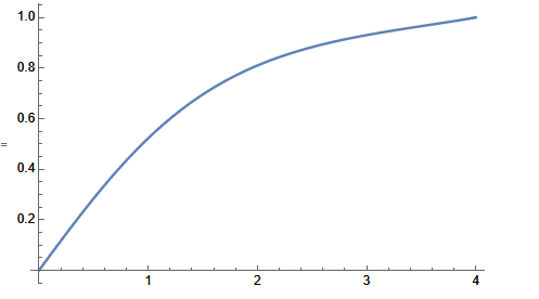
Best I could make run to is up to $x=4$

ode=1/x*D[x*f'[x],x]+(1-1/x^2)*f[x]-f[x]^3==0
k=4;
bc={f[$MachineEpsilon]==0,f[k]==1}

sol=NDSolve[{ode,bc},f,{x,$MachineEpsilon,k},
     Method->{"Shooting",
       "StartingInitialConditions"->{f[$MachineEpsilon]==0,f'[$MachineEpsilon]==1}},
        WorkingPrecision->40
 ]

enter image description here

Plot[Evaluate[f[x]/.sol],{x,0,k}]

enter image description here

There might be more tunning options to make it integrate to larger values.

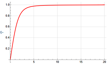
Thanks to comment below by Mariusz Iwaniuk, using f'[$MachineEpsilon]==Rationalize[1.166378991720675,0] makes it go to $x=20$.

sol = NDSolve[{ode, bc}, f, {x, $MachineEpsilon, k}, 
  Method -> {"Shooting", 
    "StartingInitialConditions" -> {f[$MachineEpsilon] == 0, 
      f'[$MachineEpsilon] == Rationalize[1.166378991720675, 0]}}, 
  WorkingPrecision -> 40]

 Plot[Evaluate[f[x] /. sol], {x, 0, k}, AxesOrigin -> {0, 0}, 
 PlotStyle -> Red, GridLines -> Automatic, 
 GridLinesStyle -> LightGray]

enter image description here

You can't solve with BC at infinity numerically. Since this BVP, you can try shooting method.

Best I could make run to is up to $x=4$

ode=1/x*D[x*f'[x],x]+(1-1/x^2)*f[x]-f[x]^3==0
k=4;
bc={f[$MachineEpsilon]==0,f[k]==1}

sol=NDSolve[{ode,bc},f,{x,$MachineEpsilon,k},
     Method->{"Shooting",
       "StartingInitialConditions"->{f[$MachineEpsilon]==0,f'[$MachineEpsilon]==1}},
        WorkingPrecision->40
 ]

enter image description here

Plot[Evaluate[f[x]/.sol],{x,0,k}]

enter image description here

There might be more tunning options to make it integrate to larger values.

Thanks to comment below by Mariusz Iwaniuk, using f'[$MachineEpsilon]==Rationalize[1.166378991720675,0] makes it go to $x=20$.

sol = NDSolve[{ode, bc}, f, {x, $MachineEpsilon, k}, 
  Method -> {"Shooting", 
    "StartingInitialConditions" -> {f[$MachineEpsilon] == 0, 
      f'[$MachineEpsilon] == Rationalize[1.166378991720675, 0]}}, 
  WorkingPrecision -> 40]

 Plot[Evaluate[f[x] /. sol], {x, 0, k}, AxesOrigin -> {0, 0}, 
 PlotStyle -> Red, GridLines -> Automatic, 
 GridLinesStyle -> LightGray]

enter image description here

Source Link
Nasser
  • 150.6k
  • 12
  • 162
  • 376

You can't solve with BC at infinity numerically. Since this BVP, you can try shooting method.

Best I could make run to is up to $x=4$

ode=1/x*D[x*f'[x],x]+(1-1/x^2)*f[x]-f[x]^3==0
k=4;
bc={f[$MachineEpsilon]==0,f[k]==1}

sol=NDSolve[{ode,bc},f,{x,$MachineEpsilon,k},
     Method->{"Shooting",
       "StartingInitialConditions"->{f[$MachineEpsilon]==0,f'[$MachineEpsilon]==1}},
        WorkingPrecision->40
 ]

enter image description here

Plot[Evaluate[f[x]/.sol],{x,0,k}]

enter image description here

There might be more tunning options to make it integrate to larger values.