Challenges with High-Order Boundary Conditions in PDEs for Beam Vibration Analysis in Mathematica

Question

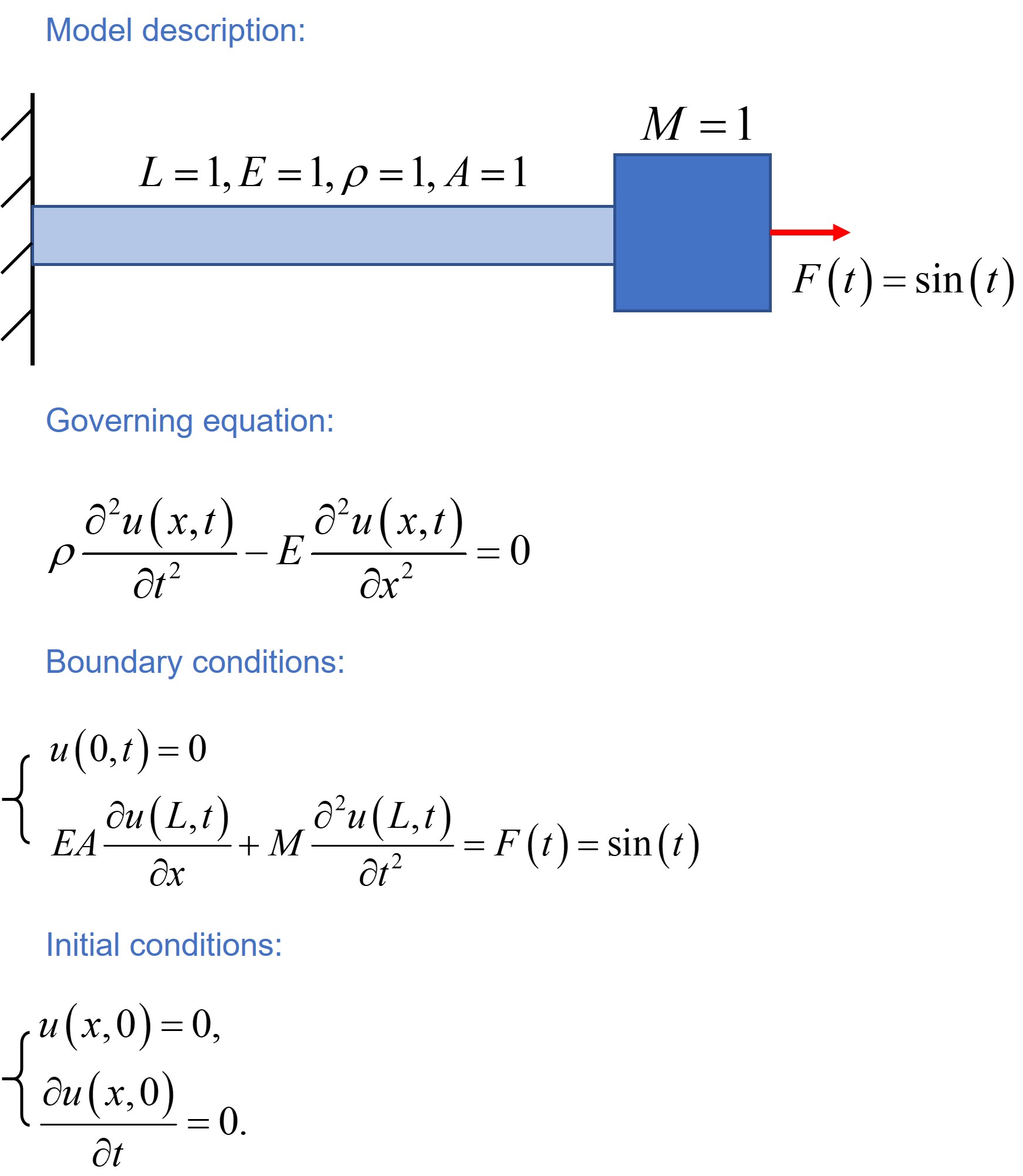
I am trying to solve a problem involving the longitudinal vibration of a beam in Mathematica. The beam is fixed at the left end and has a concentrated mass at the right end. The system is subjected to a harmonic force excitation at the right end. The following figure shows the details of my setup: And here are my codes

(* Parameters *)
L = 1;
rho = 1;
A = 1;
Emodulus = 1;
M = 1;

(* PDE for longitudinal vibration *)
pde = rho*D[u[x, t], {t, 2}] == Emodulus*D[u[x, t], {x, 2}];

(* Boundary conditions *)
bc1 = u[0, t] == 0;
bc2 = (Emodulus*A*Derivative[1, 0][u][L, t] + M*Derivative[0, 2][u][L, t]) == Sin[t];

(* Initial conditions *)
ic1 = u[x, 0] == 0;
ic2 = Derivative[0, 1][u][x, 0] == 0;

(* Solving the PDE *)
solution = NDSolve[{pde, bc1, bc2, ic1, ic2}, u[x, t], {x, 0, L}, {t, 0, 10}];

However, I encounter an error related to the boundary conditions involving the second derivative in time. I understand that introducing a second-order time derivative in the boundary condition might be problematic since it matches the order of the PDE.

Could someone help me figure out how to properly set up and solve this problem in Mathematica?

Thank you in advance!

Answer 1

This problem can be solved with the Method of Lines as follows

U[tm_] := 
 Module[{L = 1, dy = 1/10, A = 1, rho = 1, Emod = 1, M = 1}, 
  xgrid = Range[0, L, dy]; nx = Length[xgrid];
  M2 = NDSolve`FiniteDifferenceDerivative[Derivative[2], xgrid, 
     DifferenceOrder -> 4]@"DifferentiationMatrix"; 
  M1 = NDSolve`FiniteDifferenceDerivative[Derivative[1], xgrid, 
     DifferenceOrder -> 4]@"DifferentiationMatrix";
  u = Table[uu[i][t], {i, nx}]; eq = rho  D[u, t, t] - Emod  M2 . u;
  (*PDE for longitudinal vibration*)
  (*Boundary conditions*)
  eq[[1]] = D[u[[1]], t, t];
  eq[[-1]] = Emod  A  (M1 . u)[[-1]] + M  D[u[[-1]], t, t] - Sin[t];
  
  (*Initial conditions*)
  ic = Join[u, D[u, t]] /. t -> 0; eqs = Join[eq, ic];
  sol = NDSolve[Table[eqs[[i]] == 0, {i, Length[eqs]}], 
    u, {t, 0, tm}]; sol]

Function U usage for $0\le t\le 10$

s10 = U[10];

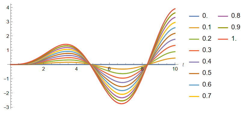
Visualization at different x=xgrid

Plot[Evaluate[u /. s10[[1]]], {t, 0, 10}, PlotLegends -> N[xgrid], 
 AxesLabel -> Automatic]