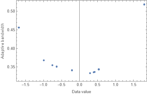
I have implemented the KDE distribution finding for a dataset. I apply the adaptive bandwidth method; I want to plot the change in bandwidth over the entire distribution. How can I do it? Thank you!

1 Answer
$\begingroup$
$\endgroup$
4
The following will give you the adaptive bandwidths that Mathematica uses:
SeedRandom[12345];
data = RandomVariate[NormalDistribution[0, 1], 10] // Sort;

α = 0.6;
kmd = KernelMixtureDistribution[data, {"Adaptive", Automatic, α}];
bw = kmd[[2, 4]]
(* {0.455945, 0.367787, 0.354622, 0.350731, 0.340984, 0.33284, 0.335444, 0.336422,
    0.343412, 0.517947}{0.455945, 0.367787, 0.354622, 0.350731, 0.340984, 0.33284,
    0.335444, 0.336422, 0.343412, 0.517947} *)
However, these bandwidths do not match what R gives (using akj in the quantreg package) which is the same as I get doing this in Mathematica with a brute force method. I'll look at that more to see if I can figure out the difference.
One can then plot those adaptive bandwidths against the data values:
ListPlot[Transpose[{data, bw}], Frame -> True,
  FrameLabel -> {"Data value", "Adaptive bandwidth"}]

