Solve Differential Equation Numerically

Question

I investigated my system and encountered differential equation such as

$y''(x) = e^{y(x)}-e^{-2y(x)}-e^{y(x)-y(x+d)}$,

where $d$ is a constant. The boundary condition is

$y'(0) = 30$

$y'(\infty)=0$.

I want to implement this in mathematica using NDSolve. Can anyone guide me as I am new to Mathematica?

Answer 1

First, consider the case d = 0:

eq0 = y''[x] - Exp[y[x]] + Exp[-2 y[x]] + 1;

with y'[0] == 30 and y'[x] == 0 asymptotically for large x. It is useful to know y[x] asymptotically as well.

ry = Solve[0 == eq0 /. y''[x] -> 0, y[x], Reals] // Flatten
(* {y[x] -> Log[Root[-1 - #1^2 + #1^3 & , 1, 0]]} *)

with the approximate value, 0.382245. Conveniently, eq0 has a first integral.

iq0 = Integrate[eq0 y'[x], x]
(* (1/2) E^(-2 y[x]) - E^y[x] + y[x] + 1/2 y'[x]^2 *)

from which {y[0], y'[0]} can be determined from the corresponding asymptotic values.

(iq0 /. y'[x] -> 0 /. ry) == (iq0 /. x -> 0 /. y'[0] -> 30);
(r0 = Solve[%, y[0], Reals] // Flatten // First
(* y[0] -> Root[{Root[-1 - #1^2 + #1^3 & , 1, 0]^2 + ... *)

with the approximate value -3.39884. eq0 now can be evaluated as an initial value problem.

NDSolveValue[{eq0 == 0, y'[0] == 30, Equal @@ r0}, y[x], {x, 0, 10}, 
    WorkingPrecision -> 46];
p0 = Plot[%, {x, 0, 10}, PlotRange -> All, AxesLabel -> {x, y}, 
    LabelStyle -> {12, Bold, Black}]

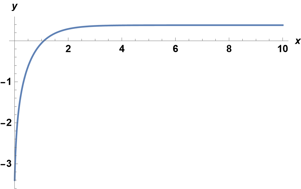
A large WorkingPrecision is needed, because the solution is a separatrix.

Now, turn to the general case, d > 0:

eq2 = y''[x] - Exp[y[x]] + Exp[-2 y[x]] + Exp[y[x] - y[x + d]];

This delay differential equation must be integrated from large x toward 0, if NDSolve is to be used. But, to do so requires a first-order expression for y[x + d] beyond the domain of integration. We already have the zero-order expression, ry. Insert this into eq2 as follows.

eq3 = FullSimplify[eq2 /. y -> Function[x, z[x] + Log[Root[-1 - #^2 + #^3&, 1, 0]]]]
(* E^(z[x] - z[d + x]) + E^z[x] Root[1 + #^2 + #^3&, 1, 0] + 
   E^(-2 z[x]) Root[-1 + # + 2 #^2 + #^3& , 1, 0] + z''[x] *)

Next, linearize the exponentials and assume that z[x] decreases exponentially for large x, which proves to be true. Thus, z[d + x] -> z[x] Exp[k d], and

FullSimplify[%/z[x] /. {(z''[x] -> k^2 z[x], 
    Exp[a_] -> 1 + a} /. z[d + x] -> z[x] Exp[k d]]
(* -E^(d k) + k^2 + Root[27 + 9 # - 6 #^2 + #^3&, 1, 0] *)

f[d_] := FindRoot[-E^(d k) + k^2 + 
    Root[27 + 9 # - 6 #^2 + #^3&, 1, 0], {k, -1.55}][[1, 2]]
Plot[f[dd], {dd, 0, 5}, AxesLabel -> {d, k}, LabelStyle -> {12, Bold, Black}]

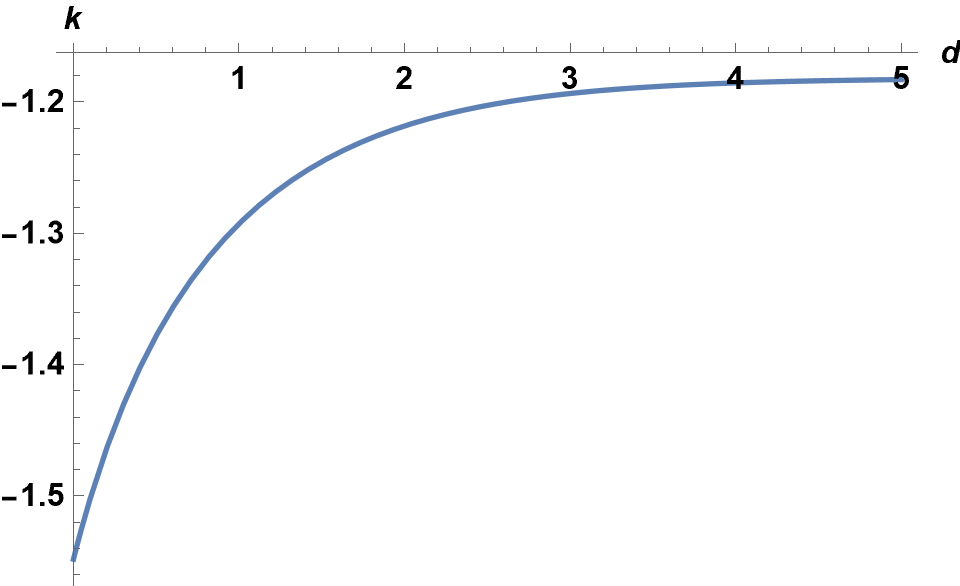
k is, evidently, a relatively weak function of d. The integration of eq3 now can be performed via shooting . (The following two blocks of code are used instead of the NDSolve Shooting option to provide greater flexibility.) As an example, choose d -> 2. (Choosing d -> 0 would, of course, recover the first curve, above.)

sp3 = ParametricNDSolveValue[{0 == eq3 /. d -> 2, 
    z[x /; x >= 10] == zm Exp[Rationalize[f[2], 0] (x - 10)], 
    z'[10] == Rationalize[f[2], 0] z[10]}, {z[x], z'[0]}, {x, 0, 10}, 
    zm, WorkingPrecision -> 46, MaxSteps -> 10^6];

Off[ParametricNDSolveValue::ihist]
FindRoot[Last[sp3[zmm]] == 30, {zmm, -83 10^-7, -82 10^-7}, 
    Evaluated -> False, WorkingPrecision -> 46];
First[sp3[zmm] /. %];
Plot[% + ry[[1, 2]], {x, 0, 10}, PlotRange -> All, PlotStyle -> Red]

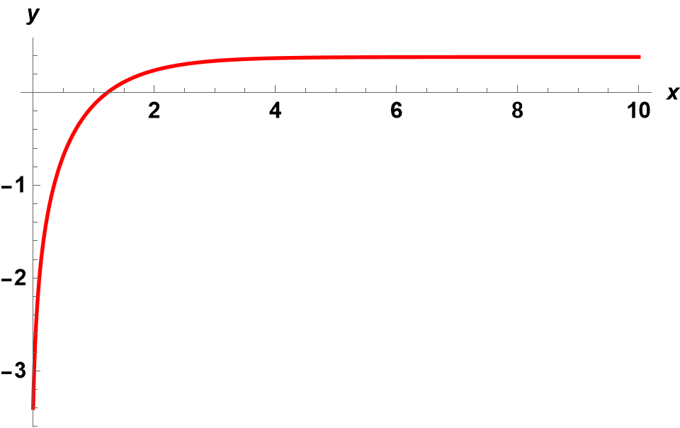
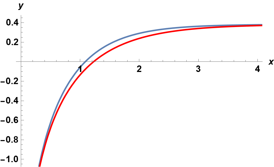
which looks a lot like the first plot, above. The largest difference occurs where the curvature is greatest.

Show[p0, p2, PlotRange -> {{0, 4}, {-1, .4}}]

Note that the FindRoot limits were obtained by trial and error, e.g.,

sp3[-80 10^-7] // Last
(* 17.32903540764105929046555619940967323250985139 *)

seeking a value near 30.