How to change NDSolve equations at every Event detection?

Question

According to this tutorial on Event Actions for NDSolve, if $x'[t]=f(t,x(t))$:

it is not possible to set the derivatives x'[t], since those are determined explicitly from the function.

In my case, I need to change the derivative function at every new event detection, as well as update the state discontinuously. (I am NOT switching between a set of a priori known equations.)

What is the "right" way to do this in Mathematica?

Below is a toy example that does not work:

buildV = Function[w,Function[t,Sin[w*t]]];
V = buildV[5*Random[]];

sol = NDSolve[{v'[t]==V'[t],
        WhenEvent[v[t]==1/2, 
          V = buildV[5*Random[]];  
          v'[t] -> V'[t];
          v[t] -> v[t]+0.05
        ],
        v[0]==V[0]},v[t],{t,0, 10}][[1]]

The output will just be a constant-frequency sinusoid, instead of one that changes frequency and jumps every time $v[t]=\frac{1}{2}$.

EDIT: Fixed a minor bug in the code where I incorrectly included a semicolon after v[t] -> v[t]+0.05. Now the plot is not a mere sinusoid, but v'[t] still does not change at any point.

EDIT: What if the input to buildV is a list of data that is expanding over time? This adaptation of Alex Trounev's answer does not work because w is not of fixed dimensionality:

buildV = Function[wLst, Function[t, Sin[Mean[wLst]*t]]]; 
vals[0]={5Random[]} 
V=buildV[vals];  

sol = NDSolve[{v'[t] == buildV[w[t]]'[t], 
        WhenEvent[v[t] == 1/2, 
          {w[t] -> Join[w[t], {5Random[]}], v[t] -> v[t] + 0.05}], 
        v[0]==V[0], w[0]==vals[0]}, 
        {v, w}, {t, 0, 10}, DiscreteVariables -> w][[1]];

My full example:

Legendre[n_,t_]=LegendreP[n-1,(2t-1)]*Sqrt[2(n-1)+1];
p[n_,t_]=Legendre[n,Exp[-t]]*HeavisideTheta[t];
\[Omega][t_]=Exp[-t];
K[n_,t_]=p[n,t]*\[Omega][t];

func[t_]=Sin[2Pi*t];
d=2;
T=3;

f=Function[\[Tau],Evaluate@Table[
Integrate[func[t]*p[k,t-\[Tau]]*\[Omega][t-\[Tau]],{t,\[Tau],\[Infinity]},Assumptions->\[Tau]>=0]
,{k,d}]];

interactions=Function[\[CapitalDelta],Evaluate@Table[
Integrate[K[i, t]*K[j, t+\[CapitalDelta]], {t, 0, \[Infinity]},Assumptions->\[CapitalDelta]>=0]
,{i,d},{j,d}]];

buildV=Function[spkList,
Function[\[Tau],Evaluate[
f[\[Tau]]-Table[
Total[HeavisideTheta[\[Tau]-#[[2]]]*#[[3]]*interactions[\[Tau]-#[[2]]][[m,#[[1]]]]&/@spkList]
,{m,d}]]]];

eps=10.^-5;
tStart=0;
spikes=Table[{i,tStart-eps,f[tStart-eps][[i]]},{i,d}];(*{{idx,time,weight}}*) 
V=buildV[spikes];

sol=NDSolve[{{v1'[t],v2'[t]}==V'[t],
WhenEvent[v1[t]==1/4,
spikes= Join[spikes,{{1,t,1}}];
V=buildV[spikes];
(*{v1[t],v2[t]}->V[t]
{v1'[t],v2'[t]}->V'[t]*)
],
WhenEvent[v1[t]==-1/4,
spikes= Join[spikes,{{1,t,-1}}];
V=buildV[spikes];
(*{v1[t],v2[t]}->V[t]
{v1'[t],v2'[t]}->V'[t]*)
],
WhenEvent[v2[t]==1/4,
spikes= Join[spikes,{{2,t,1}}];
V=buildV[spikes];
(*{v1[t],v2[t]}->V[t]
{v1'[t],v2'[t]}->V'[t]*)
],
WhenEvent[v2[t]==-1/4,
spikes= Join[spikes,{{2,t,-1}}];
V=buildV[spikes];
(*{v1[t],v2[t]}->V[t]
{v1'[t],v2'[t]}->V'[t]*)
],
{v1[tStart],v2[tStart]}==V[tStart]},
{v1[t],v2[t]},{t,tStart, T}][[1]]

Answer 1

We can use discrete variable to control w as follows

buildV = Function[w, Function[t, Sin[w*t]]];
sol = NDSolve[{{v'[t] == buildV[w[t]]'[t], v[0] == 0, 
w[0] == 5 RandomReal[]}, 


WhenEvent[v[t] == 1/2, {w[t] -> 5 RandomReal[],
     v[t] -> v[t] + 0.05}]}, {v, w}, {t, 0, 10}, 
  DiscreteVariables -> w]

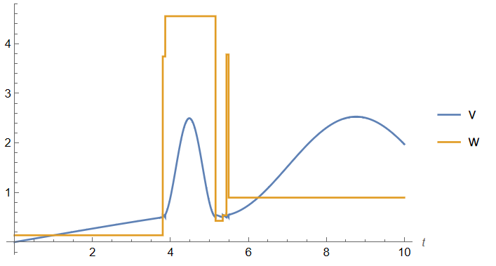
Visualization

Plot[Evaluate[{v[t], w[t]} /. sol[[1]]], {t, 0, 10}, 
 PlotPoints -> 200, PlotRange -> All, PlotLegends -> {"v", "w"}, 
 AxesLabel -> Automatic] 

Update 1. Second toy example can be solved with using "Do" loop as follows

Unprotect[HeavisideTheta]; 
HeavisideTheta[0.0] = 1; Protect[HeavisideTheta];

Legendre[n_, t_] = LegendreP[n - 1, (2 t - 1)]*Sqrt[2 (n - 1) + 1];
p[n_, t_] = Legendre[n, Exp[-t]]*HeavisideTheta[t];
\[Omega][t_] = Exp[-t];
Kk[n_, t_] = p[n, t]*\[Omega][t];
func[t_] = Sin[2 Pi*t];
d = 2;
T = 3;
f = Function[\[Tau], 
   Evaluate@
    Table[Integrate[
      func[t]*p[k, t - \[Tau]]*\[Omega][
        t - \[Tau]], {t, \[Tau], \[Infinity]}, 
      Assumptions -> \[Tau] >= 0], {k, d}]];


interactions = 
  Function[\[CapitalDelta], 
   Evaluate@
    Table[Integrate[
      Kk[i, t]*Kk[j, t + \[CapitalDelta]], {t, 0, \[Infinity]}, 
      Assumptions -> \[CapitalDelta] >= 0], {i, d}, {j, d}]];

buildV = 
  Function[spkList, 
   Function[\[Tau], 
    Evaluate[
     f[\[Tau]] - 
      Table[Total[
        HeavisideTheta[\[Tau] - #[[2]]]*#[[3]]*
           interactions[\[Tau] - #[[2]]][[m, #[[1]]]] & /@ 
         spkList], {m, d}]]]];


tStart = 0;
spikes = Table[{i, tStart - eps, f[tStart - eps][[i]]}, {i, d}]; V = 
 buildV[spikes];


tS[0] = tStart; spike[0] = spikes; 
spk[i_] := {{{1, tS[i], 1}}, {{1, tS[i], -1}}, {{2, tS[i], 1}}, {{2, 
    tS[i], -1}}}; Do[{V1[i], V2[i]} = 
  NDSolveValue[{{v1'[t], v2'[t]} == V'[t], 
    WhenEvent[v1[t] == 1/4, {tS[i] = t, j = 1}; "StopIntegration"], 
    WhenEvent[v1[t] == -1/4, {tS[i] = t, j = 2}; "StopIntegration"], 
    WhenEvent[v2[t] == 1/4, {tS[i] = t, j = 3}; "StopIntegration"], 
    WhenEvent[v2[t] == -1/4, {tS[i] = t, j = 4}; "StopIntegration"],
    WhenEvent[Abs[v2[t]] == 1/4, tS[i] = t; 
     "StopIntegration"], {v1[tS[i - 1]], v2[tS[i - 1]]} == 
     V[tS[i - 1]]}, {v1, v2}, {t, tS[i - 1], tS[i - 1] + 1}]; 
 spike[i] = Join[spike[i - 1], spk[i][[j]]]; 
 V = Evaluate[buildV[spike[i]]];, {i, 10}];

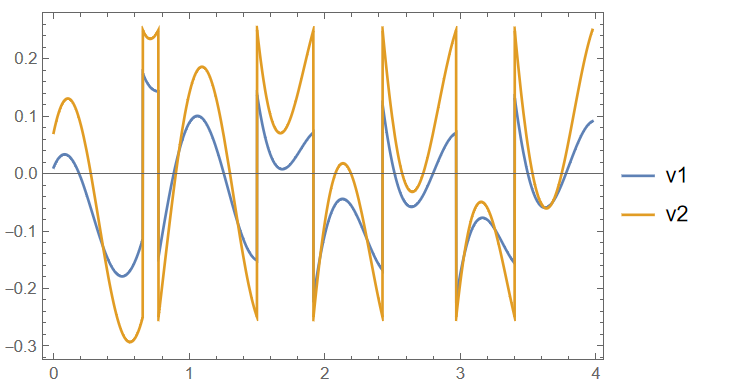
Visualization

VV1 = Piecewise[
  Table[{V1[i], tS[i - 1] <= t < tS[i]}, {i, 10}]]; VV2 = 
 Piecewise[Table[{V2[i], tS[i - 1] <= t < tS[i]}, {i, 10}]];

Plot[{VV1[t], VV2[t]}, {t, tS[0], tS[10]}, Frame -> True, 
 PlotLegends -> {"v1", "v2"}]