The default type of interpolation produced by NDSolve stores for each discrete step the domain abscissa $x_j$, the function value $y(x_j)$, and the derivative values $y^{k}(x_j)$ up to the order of the ODE. In the OP's example, the derivatives stored are $y'(x_j)$ and $y''(x_j)$.
The data structure inside InterpolatingFunction[<...>] is shown in
What's inside InterpolatingFunction[{{1., 4.}}, <>]?
and in the code toward the end of this answer,
Interpolating data with a step.
Part 4 contains the function and derivative data for each step. It is stored in a flat array of the form
(*
{y[x0], y'[x0],..., Derivative[k][y][x0],
 y[x1], y'[x1],..., Derivative[k][y][x1],
 ...}
*)
The data also contains offsets that indicate where each function/derivative value unit ends. When the order of the ODE is k = 2, there are three values per unit y, y', y''.
yIFN = y /. First[s];
yIFN[[4]]
(*
{Developer`PackedArrayForm,       (* type of data *)
 {0, 3, 6, 9, ... 1407},          (* offsets *)
 {1.`, 0.`, -0.8414709848078965`, (* function/derivative values *)
  0.9999999750347968`, -0.00014493961665665655`, -0.8414709503116456`,
  0.9999999251043933`, -0.00028987922142966306`, -0.8414708813191469`,
  ...,
  0.9989990862203024`,  0.04101857645543858`,    -0.8400880807981383`}}
*)
The argument "ValuesOnGrid" gives a slice of this data for each of the derivatives computed by NDSolve (i.e., y, y', y'' in the OP example):
yIFN["ValuesOnGrid"][[{1, 2, 3, -1}]]
yIFN'["ValuesOnGrid"][[{1, 2, 3, -1}]]
yIFN''["ValuesOnGrid"][[{1, 2, 3, -1}]]

(*       y[x]         |           y'[x]            |         y''[x]
{1.`,                 | {0.`,                      | {-0.8414709848078965`,
 0.9999999750347968`, |  -0.00014493961665665655`, |  -0.8414709503116456`,
 0.9999999251043933`, |  -0.00028987922142966306`, |  -0.8414708813191469`,
 0.9989990862203024`} |  0.04101857645543858`}     |  -0.8400880807981383`}
*)
Note these values match the data shown for yIFN[[4]]. If you ask for higher derivatives, they are computed from the interpolation. We have 6 values total for each interpolation interval (3 at each end point). They determine a degree 5 interpolant. Derivatives of order 6 and higher are zero.
Derivative[3][yIFN]["ValuesOnGrid"][[{1, 2, 3, -1}]]
Derivative[4][yIFN]["ValuesOnGrid"][[{1, 2, 3, -1}]]
Derivative[5][yIFN]["ValuesOnGrid"][[{1, 2, 3, -1}]]
Derivative[6][yIFN]["ValuesOnGrid"][[{1, 2, 3, -1}]]
(*
{-146559., -146559., -146559., ..., -0.0565191}
{5.10523*10^9, -5.10523*10^9, -5.10523*10^9, ..., 1.1701}
{-5.92786*10^13, -5.92786*10^13, -5.92786*10^13, ..., 0.366953}
{0., 0., 0., ..., 0.}
*)
What looks like numerical instability is probably due to the small step sizes at the beginning:
Differences[yIFN["Grid"]][[{1, 2, 3, -1}]]
(*  {{0.000172246}, {0.000172246}, {0.00382697}, {0.0971486}}  *)

Derivative[5][yIFN] // ListLinePlot[#, PlotRange -> All] &
Derivative[5][yIFN] // ListLinePlot
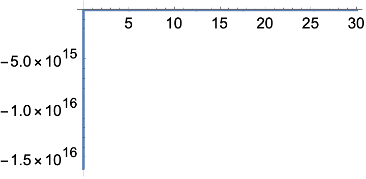
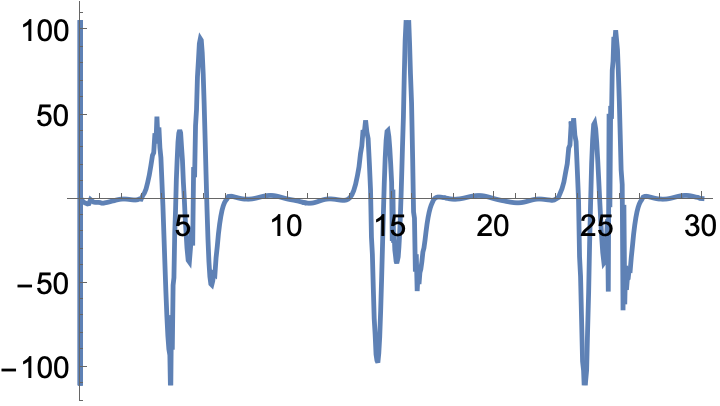
Update
Another thing worth mentioning is that only one thing is changed in yIFN when it is differentiated. The order of the derivative is changed in the InterpolatingFunction structure.
yIFN''''[[4]] === yIFN[[4]]
(*  True  *)
The derivative of the interpolation may be inspected by Part or via the "DerivativeOrder" method:
yIFN[[2, 6]]
yIFN''[[2, 6]]
yIFN''''[[2, 6]]
(*
  0
  {2}
  {4}
*)

yIFN''''["DerivativeOrder"]
(*  Derivative[4]  *)
Related Q&A:
These deal with variations due to InterpolationOrder -> All:



NDSolve." - then you need to actually provide the relevant equations for the derivatives, sincey'[x]is by necessity directly differentiating theInterpolatingFunction. $\endgroup$Interpolationcan construct anInterpolatingFunctionthat reproduces the values of derivatives as well as those of the function itself. Since this capability exists, I would think thatNDSolvewould provide that information in itsInterpolatingFunctionoutput. But this is speculation on my part. As an aside, you could useNDSolveValue[yourEquation, {y, y', y''}, {x, 0, 30}]to get separateInterpolatingFunctionobjects representing the function and each of its derivatives, right from withinNDSolve. $\endgroup$