Writing code for a diagram

Question

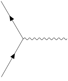
Could anyone please help in writing the code for the following diagram in Mathematica?

Note: I want a simple code in Mathematica without using an external package.

Answer 1

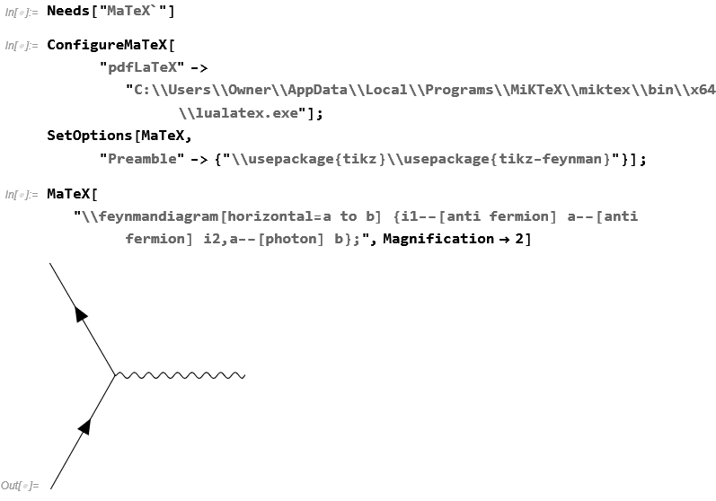
Use MaTeX?

MaTeX["\\feynmandiagram[horizontal=a to b] {i1--[anti fermion] 
a--[anti fermion] i2,a--[photon] b};", Magnification -> 2]

Note that this needs lualatex and not pdflatex, which is the default used by MaTeX. I do not know how to tell MaTeX to use lualatex instead of pdflatex as the default compiler, so I cheated a little. You need to do the following before issuing the above command.

Needs["MaTeX`"]

ConfigureMaTeX["pdfLaTeX" ->"C:\\Users\\Owner\\AppData\\Local\\Programs\\MiKTeX\\miktex\\bin\\x64\\lualatex.exe"];

SetOptions[MaTeX, "Preamble" -> {"\\usepackage{tikz}\\usepackage{tikz-feynman}"}]

And now you can issue the command.

There is also FeynCalc which is is a Mathematica package for symbolic evaluation of Feynman diagrams but I never used it myself and do not have it installed. You could look at it.

There is also old FeynArts https://library.wolfram.com/infocenter/Articles/1638/ this paper describes the Mathematica package FeynArts used for the generation and visualization of Feynman diagrams

Update

Note: I want a simple code in Mathematica without using an external package.

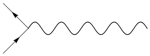
The above was added later. Here is a quick plot using standard Mathematica Graphics. Feel free to adjust as needed

Graphics[{First@Plot[1/2 Sin[3*x], {x, 0, 3*Pi}, PlotStyle -> Black],
  {Arrowheads[{0, 0, 0.05, 0}], Arrow[{{0, 0}, {-2, 2}}]},
  {Arrowheads[{0, 0, 0.05, 0}], Arrow[{{-2, -2}, {0, 0}}]}}]

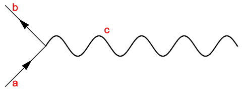
Also could you please label say a, b, c all of the three lines

One option is to use Textand adjust the location as needed.

Graphics[{First@
   Plot[1/2 Sin[3*x], {x, 0, 3*Pi}, 
    PlotStyle -> Black], {Arrowheads[{0, 0, 0.05, 0}], 
   Arrow[{{0, 0}, {-2, 2}}]}, {Arrowheads[{0, 0, 0.05, 0}], 
   Arrow[{{-2, -2}, {0, 0}}]},
  Text[Style["a", Red, 16], {-1.5, -1.8}],
  Text[Style["b", Red, 16], {-1.5, 1.9}],
  Text[Style["c", Red, 16], {3, .8}]
  }
 ]

Answer 2

The arrows can be drawn using "Arrow" and for the wiggly line we use a Bezier curve.

For the Bezier curve some control points are needed. We choose control points at a distance of +/-0.5 above/below the y and 0.5 spaced along the x axis:

dx = 0.3;
dy = 0.5;
n = 7;
ctrl = Table[{i dx, Mod[i, 3, -1] dy}, {i, n}]

With this we can now draw the diagram:

gr=Graphics[{Thickness[0.01]
  , Arrowheads[0.1], Arrow[{{-1, -1}, {0, 0}}, 0.5], 
  Line[{{-1, -1}, {0, 0}}]
  , Arrow[{{0, 0}, {-1, 1}}, 0.5], Line[{{-1, 1}, {0, 0}}]
  , BezierCurve[Join[{{0, 0}}, ctrl, {{++n dx, 0}}]]
  }]

Answer 3

Here is a part of my package for performing calculations with Feynman diagrams:

1.1 Define a set of Feynman diagrams

Clear[f, G, V]
f[0, 1][a_, b_, c_, d_] = 
 diag[g[a, i[1]], g[b, i[2]], g[i[1], c], g[i[2], d], v[i[1], i[2]]]
f[0, 2][a_, b_, c_, d_] = 
 diag[g[a, i[1]], g[b, i[2]], g[i[1], d], g[i[2], c], v[i[1], i[2]]]

1.2 Define a plotting function

pic[diag[x__]] := Module[{i, j, k},
    Graph[List[x] /. {g[i_, j_] -> DirectedEdge[j, i],
                        v[j_, k_] -> UndirectedEdge[j, k]},
                    VertexLabels -> "Name",
                    PlotTheme -> "Business",
                    ImageSize -> 300, ImagePadding -> 10,
                    VertexLabelStyle -> Directive[Black, 11],
                    GraphHighlight -> 
    Cases[List[x], v[i_, j_] -> UndirectedEdge[i, j]]]]

1.3 Depict 2 two-particle Green's functions to the first order in the Coulomb interaction

pic /@ {f[0, 1][a, b, c, d], f[0, 2][a, b, c, d]}

Let us do a bit more complicated stuff. We re-sum two-particle diagrams in the $T$-matrix (particle-particle channel) fashion

2.1 Define functions for contracting diagrams

vlist[diag[x__]] := Union[Flatten[Apply[List, List[x], 1]]]
contract[x__, vC_] := Module[{dlist, vtab, vE, vI, dj, rules, ka},
  dlist = List[x];
  (* replace contracted indices *)
  
  rules = Table[vC[[j]] -> i[0, j], {j, Length[vC]}];
  dlist = dlist /. rules;
  (* rename internals *)
  dlist = Table[dj = dlist[[j]];
    rules = Flatten[Cases[vlist[dj], i[ka_] -> {i[ka] -> i[j, ka]}]];
    dj /. rules, {j, Length[dlist]}];
  (*Combine diagrams together*)
  
  dlist = Apply[diag, Flatten[List @@@ dlist]];
  (* Rename internals*)
  vI = Cases[vlist[dlist], i[__]];
  dlist /. Rule @@@ Transpose[{vI, i /@ Ordering[vI]}]
  ]

2.2 Define $T$-matrix diagrams

f[1, 2][a_, b_, c_, d_] = 
  contract[f[0, 1][p, q, c, d], V[p, q], G[a, p], G[b, q], {p, q}];
f[2, 2][a_, b_, c_, d_] = 
  contract[f[1, 2][p, q, c, d], V[p, q], G[a, p], G[b, q], {p, q}];
f[3, 2][a_, b_, c_, d_] = 
  contract[f[2, 2][p, q, c, d], V[p, q], G[a, p], G[b, q], {p, q}];

2.3 and plot the result

f[3, 2][a, b, c, d] // pic