Spurious poles in a gain plot (due to machine precision or complex numbers?)

Question

I have the following plot that I like to make. It details the gain of an amplifier.

Clear["Global`*"]

ϕ0 = 2.07;(*fWb*)
fp = 7.5;
ωp = 2 π*fp;(*GHz*)
ωs = 2 π*fs;
ωi = (2*ωp - ωs);
a = 10;(*micro-meters*)
LL = 1670*10^-3;(*nH*)
Ij = ϕ0/(2 π*LL);
Ip = 0.5*Ij;
zchar = 50;
CC = 667*10^-6;(*nF*)
Cj = 9.6*10^-6;(*nF*)
x = NN*a;

RR = 3.182*10^3;(*Ohms*)


kp = (a^2 ωp (I + 2 CC RR ωp) + √(1/LL a^2 ωp (I + 2 CC RR ωp)^2 (a^2 LL ωp - 2 RR (-I + 2 CC RR ωp) (-1 + Cj LL ωp^2))))/(a^2 (ωp + 4 CC^2 RR^2 ωp^3));

ks = (a^2 ωs (I + 2 CC RR ωs) + √(1/LL a^2 ωs (I + 2 CC RR ωs)^2 (a^2 LL ωs - 2 RR (-I + 2 CC RR ωs) (-1 + Cj LL ωs^2))))/(a^2 (ωs + 4 CC^2 RR^2 ωs^3));

ki = (a^2 ωi (I + 2 CC RR ωi) + √(1/LL a^2 ωi (I + 2 CC RR ωi)^2 (a^2 LL ωi - 2 RR (-I + 2 CC RR ωi) (-1 + Cj LL ωi^2))))/(a^2 (ωi + 4 CC^2 RR^2 ωi^3));

Ap0 = (Ip*zchar)/ωp;

αpeff = Simplify[1/I*((kp (-2 I + kp))/(1 + kp (I + 2 CC RR ωp)) + (kp (-2 I + kp + 2 I CC kp RR ωp))/(16 Ij^2 LL^2 (-1 + Cj LL ωp^2) (1 + kp (I + 2 CC RR ωp)))*Abs[Ap0]^2)];

αseff = Simplify[1/I*((ks (-2 I + ks))/(1 + ks (I + 2 CC RR ωs)) + (ks (-2 I + ks + 2 I CC ks RR ωs))/(8 Ij^2 LL^2 (-1 + Cj LL ωs^2) (1 + ks (I + 2 CC RR ωs)))*Abs[Ap0]^2)];

αieff = Simplify[1/I*((ki (-2 I + ki))/(1 + ki (I + 2 CC RR ωi)) + (ki (-2 I + ki + 2 I CC ki RR ωi))/(8 Ij^2 LL^2 (-1 + Cj LL ωi^2) (1 + ki (I + 2 CC RR ωi)))*Abs[Ap0]^2)];

κseff = Simplify[1/I*((ks (-2 I + ks + 2 I CC ks RR ωs))/(16 Ij^2 LL^2 (-1 + Cj LL ωs^2) (1 + ks (I + 2 CC RR ωs)))*Ap0^2)];

κieff = Simplify[1/I*(ki (-2 I + ki + 2 I CC ki RR ωi))/(16 Ij^2 LL^2 (-1 + Cj LL ωi^2) (1 + ki (I + 2 CC RR ωi)))*Ap0^2];

κistareff = Simplify[ComplexExpand[Conjugate[κieff]]];

ΔkL = 2 kp - ks - ki;
ΔkNL = 2 αpeff - αseff - αieff;
Δk = ΔkL + ΔkNL;
g = √((κseff*κistareff) - (Δk/2)^2);

newlhtlgain = Abs[Cosh[g*x]]^2 + Abs[Δk/(2 g)*Sinh[g*x]]^2 + I/2*(Conjugate[Δk/g*Sinh[g*x]]*Cosh[g*x] - Δk/g*Sinh[g*x]*Conjugate[Cosh[g*x]]);

Plot[10*Log10[Chop[newlhtlgain /. {NN -> 1000}]], {fs, 0, 15}, AxesOrigin -> {0, 0}, PlotRange ->{All, {0, 30}}]

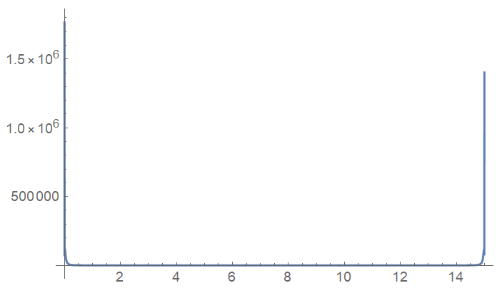
At the output, which shows the gain as a function of frequency, I get something like this

where my gain blows up at the beginning and end of the x-axis. However, if I zoom into the range of y-axis that I'm interested in. Namely, 0 to 30

Plot[10*Log10[Chop[newlhtlgain /. {NN -> 1000}]], {fs, 0, 15}, AxesOrigin -> {0, 0}, PlotRange -> {All, {0, 30}}]

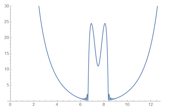
I get something like this

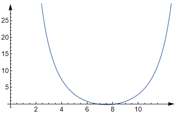
where it shows the correct gain profile in the x-axis range of 6.5 to 8.4, before the tail ends start to grow. In general, this shouldn't happen and the tail ends decay with the ripples. Why is this happening?

Edit: I suspect that this has to do with the way I'm writing my expressions for complex numbers. It would appear that printing newlhtlgain/.{NN->1000, fs->3} gives something like 57.5678-3.747*10^-16I. It's clear that the imaginary component is not suppose to be there, so using the Chop function should help. However, that doesn't change the overall shape of the plot at all.

Answer 1

How about increasing the precision of your numbers? In Mathematica you can do this by using `, like this: 10.`50, which means number 10.000... has 50 correct digits.

\[Phi]0 = 2.07`50;(*fWb*)
fp = 7.5`50;
\[Omega]p = 2 \[Pi]*fp;(*GHz*)
\[Omega]s = 2 \[Pi]*fs;
\[Omega]i = (2*\[Omega]p - \[Omega]s);
a = 10;(*micro-meters*)
LL = 1670*10^-3;(*nH*)
Ij = \[Phi]0/(2 \[Pi]*LL);
Ip = 1/2*Ij;
zchar = 50;
CC = 667*10^-6;(*nF*)
Cj = 9.6`50*10^-6;(*nF*)
x = NN*a;
RR = 3.182`50*10^3;(*Ohms*)

The resulting plot is below. Unsure however why your gain would be negative near (7,8).