Solving coupled ODE by analyzing solution near zero

Question

This question is related to an earlier question I had asked, regarding coupled first order odes. I'll add the system of odes with their boundary conditions again here. .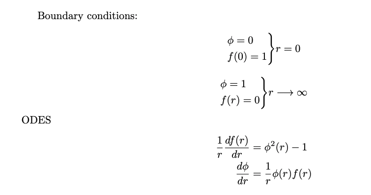

The comments for the previous post were helpful.

I was wondering if the following could be done. Start with the first two boundary conditions and impose them at $r=0$, namely,$ \phi(0)=0 $and $f(0)=1$. We know how the functions behave close to zero: $\phi(r) = c_1*r+c_2*r^2+... $and $f(r)= 1+f_1 * r+ f_2*r^2+..$. If we perform this Taylor expansion around zero and plug it into the coupled system, we generate a recursion relation between the coefficients $c_n$ and $f_n$. All these coefficients can be expressed as a function of $c_1$. I tried this by hand upto $O(r^5)$. If we consider the value of these Taylor expanded functions at some $r=0.01$ and use that as the initial condition for my system of ODEs, can I try and sweep over the free parameter $c_1$ so as to get the desired behaviour I want.

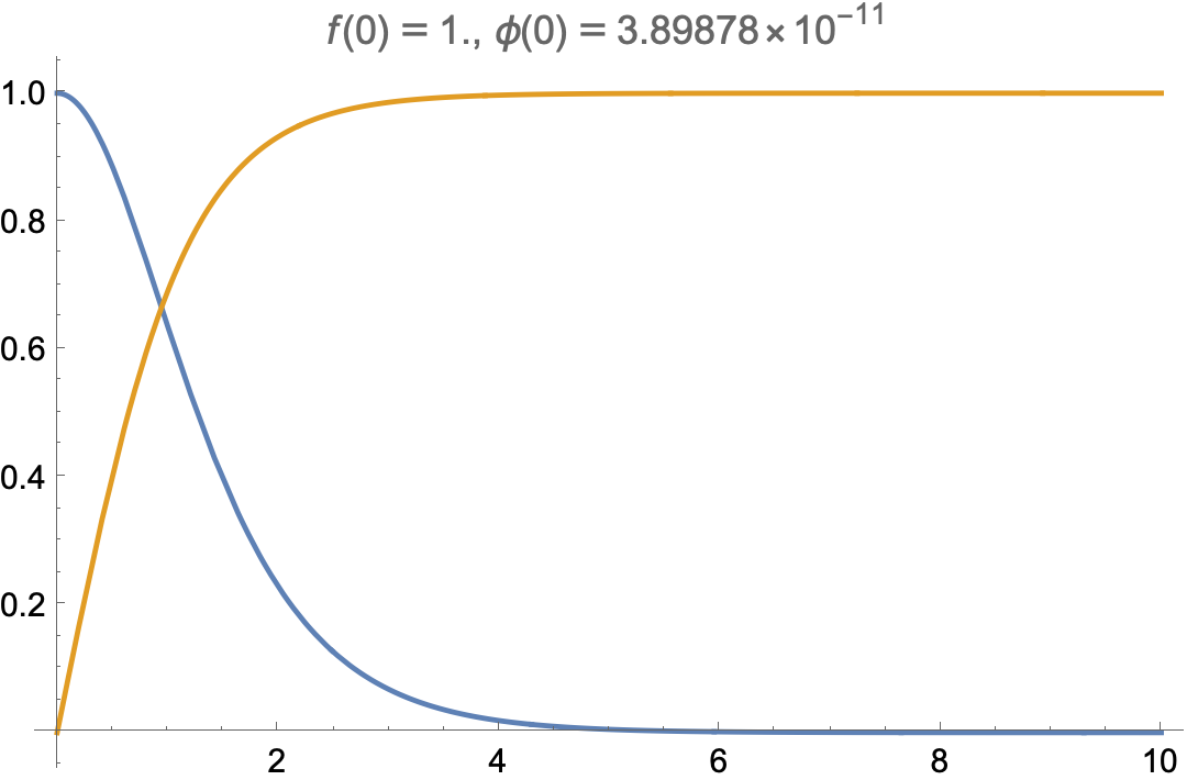
I'm attaching the desired graphs which satisfy all four conditions 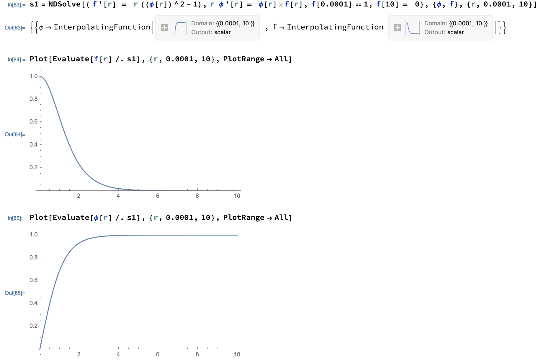. I've been trying to do this "sweeping" on Mathematica in the following manner. The $c$ used in the code is the same as the $c_1$ coefficient I'm referring to here in the text :

f[c_, r_] := 1 - (1/2) r^2 + (c^2/4  ) r^4 - (c^2/12) r^6
\[Phi][c_, r_] := c*r - (c/4) r^3 + ((c^3/16) + c/32) r^5
soln = ParametricNDSolve[{f'[r] == 
    r  (\[Phi][r]^2 - 1), \[Phi]'[r] ==  f[r] \[Phi][r]/r, 
   f[0.1] == f[c, 0.1], \[Phi][0.1] == \[Phi][c, 0.1]}, {\[Phi], 
   f}, {r, 0.1, 10}, c]

and

Plot[Evaluate[Table[f[c][r] /. soln, {c, 0.84, 0.85, 0.001}]], {r, 
  0.1, 10}, PlotRange -> {0, 2}]
Plot[Evaluate[
  Table[\[Phi][c][r] /. soln, {c, 0.84, 0.85, 0.001}]], {r, 0.1, 10}, 
 PlotRange -> {0, 2}]

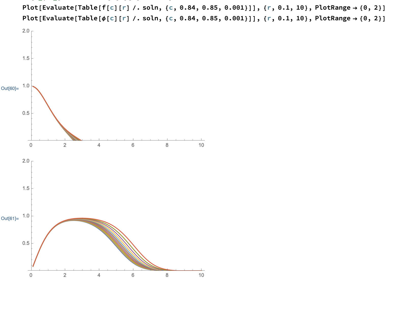
For c lying between 0.84 and 0.85, I get the following graphs:

and for c lying between 0.85 and 0.86 I get the following graphs:

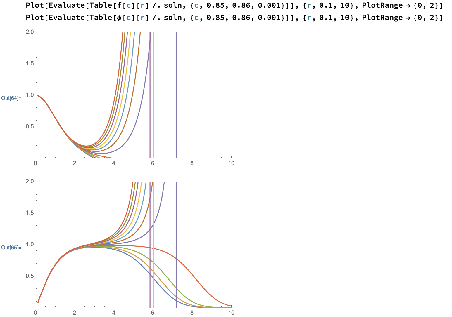
So I know that c should lie somewhere in this regime but I do not know of a way to isolate the number. Also, from fig.3, we can see that $\phi(r)$ approaches its desired behaviour better than $f(r)$.Unfortunately, I do not know of an efficient way to get my desired graphs by varying c.

Answer 1

Instead of starting at the singular point, why not start at the other end?

One trick to dealing with a singular point in the formula for a derivative is to use Piecewise to give the numeric value of the derivative at the singular point and use the formula elsewhere. The trouble here is that we don't seem to know the derivative at r == 0, but we could try to solve for it. One nice thing about the ODE system is that it's likely going to force $\phi(r)\rightarrow0$ as $r\rightarrow0$. So what we'll do is make a guess what $\phi'(0)$ will be -- I don't believe it has to be very close, since it will only make a difference in the last integration step -- and then iteratively adjust the initial condition at r == 10 to shoot for the boundary condition at r == 0 and update the derivative value after each step. (We estimate the derivative $\phi'(0)$ by the solution at r == 10^-6 because the derivative at zero is set equal to the current estimate and would never change. This introduces a small error, but singular points are difficult.)

ClearAll[f, ϕ, r, c, ϕp];
sys = {
   f'[r] == r (ϕ[r]^2 - 1),
   ϕ'[r] == Piecewise[{
      {f[r] ϕ[r]/r, r > 0}
      }, ϕp],  (* value at r == 0 *)
   f[10] == f0, ϕ[10] == ϕ0};
ϕp = 1.; (* educated(?) guess; set AFTER sys *)
obj[a0_?NumericQ] := Block[{a = a0, b = 1 - 0 1*^-8},
   soln = 
    ParametricNDSolve[sys, {ϕ, f}, {r, 0, 10}, {f0, ϕ0},
     AccuracyGoal -> 12, (* makes it strive for ϕ[0] == 0 *)
     Method -> {"Extrapolation", Method -> "LinearlyImplicitEuler"},
     InterpolationOrder -> All];
   ϕp = D[ϕ[a, b][r] /. soln, r] /. 
     r -> (ϕ[a, b]["Domain"] /. soln)[[1, 1]] + 1*^-6;
   f[a, b][0] /. soln
   ];
logf0 = a /. FindRoot[obj[Exp@a] == 1, {a, -5, -6}] (* Exp keeps parameter >0 *)

(*  -11.3726  *)

Block[{a = Exp@logf0, b = 1 - 0 1*^-8},
 Plot @@ {{f[a, b][r], ϕ[a, b][r]} /. soln, 
   Flatten@{r, f[a, b]["Domain"] /. soln},
   PlotLabel -> 
    Row[{f[0] == (f[a, b][0] /. soln), 
      ", ", ϕ[0] == (ϕ[a, b][0] /. soln)}]}
 ]