NDSolve of a stiff system of ODE's

Question

I am trying to solve numerically the following set of differential equations

eqs = { 
D L^2 c'[y] - L my[y] == 0, 
D L^2 my''[y] - L (Qyy'[y] + c'[y]/3) - my[y] == 0, 
D L^2 Qyy''[y] - (4/15) L my'[y] - Qyy[y] == 0,

c[-1] - L my[-1] - 1/(3 D) == 0,
D L^2 my'[-1] - L (Qyy[-1] + (1 + c[-1])/3) == 0, 
D L^2 my'[1] - L (Qyy[1] + (1 + c[1])/3) == 0,
D L^2 Qyy'[-1] - (4/15) L my[-1] == 0, 
D L^2 Qyy'[1] - (4/15) L my[1] == 0
}

What I am actually interested is the solution to above set of equations for the parameters D and L being from the interval (0,1). For not too small values of D, and L, one can just simply use NDSolve without any further problems to obtain an accurate solution.

For small values of D and L, for example D = 1/2, and L = 1/10, the solution is very stiff close to the boundaries y = - 1, and 1, so that the solution is problematic

pars = {D -> 1/2, L -> 1/10};
sol = NDSolve[eqs /. pars, {c, my, Qyy}, {y, -1, 1}];
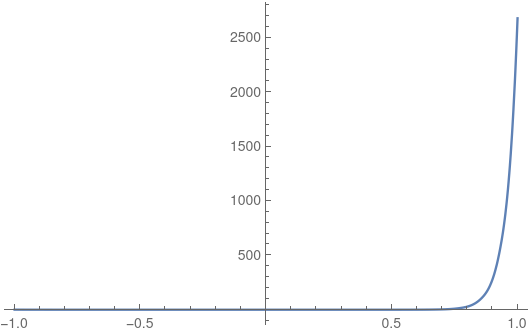
Plot[c[y] /. sol, {y, -1, 1}, PlotRange -> All]

NDSolve::bvluc: The equations derived from the boundary conditions are numerically ill-conditioned. The boundary conditions may not be sufficient to uniquely define a solution. If a solution is computed, it may match the boundary conditions poorly.

NDSolve::berr: The scaled boundary value residual error of 2.9891304910534367`*^10 indicates that the boundary values are not satisfied to specified tolerances. Returning the best solution found.

First approach

My first idea was to solve this problem using StiffnessSwitching method, but this does not automatically solve the problem

pars = {D -> 1/2, L -> 1/10};
sol = NDSolve[eqs /. pars, {c, my, Qyy}, {y, -1, 1}, 
   Method -> "StiffnessSwitching"];
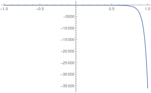
Plot[c[y] /. sol, {y, -1, 1}, PlotRange -> All]

NDSolve::bvluc: The equations derived from the boundary conditions are numerically ill-conditioned. The boundary conditions may not be sufficient to uniquely define a solution. If a solution is computed, it may match the boundary conditions poorly.

NDSolve::berr: The scaled boundary value residual error of 1.631995982197461`*^8 indicates that the boundary values are not satisfied to specified tolerances. Returning the best solution found.

I assume the problem is related to the mesh that StiffnessSwitching method is using. I could in principle set MaxStepSize -> 0.001, but I guess this makes the whole StiffnessSwitching method useless if the MaxStepSize is smaller than the step size used in StiffnessSwitching. Is there a different way of approaching this problem? Is there a way of telling mathematica to use a finer mesh, but to preserve the uneven distribution of points convenient for dealing with stiff functions?

Second approach

I also tried to solve this problem using spectral methods. If I understand the documentation correctly (https://reference.wolfram.com/language/tutorial/NDSolveMethodOfLines.html) the following code should solve the equations on the Chebyshev grid, but the result does not seem to differ from the original approach that was done without specifying any Method at all

pars = {D -> 1/2, L -> 1/10};
points = 80;
sol = NDSolve[eqs /. pars, {c, my, Qyy}, {y, -1, 1}, 
   Method -> {"MethodOfLines", 
     "SpatialDiscretization" -> {"TensorProductGrid", 
       "DifferenceOrder" -> "Pseudospectral", "MaxPoints" -> points, 
       "MinPoints" -> points}}];
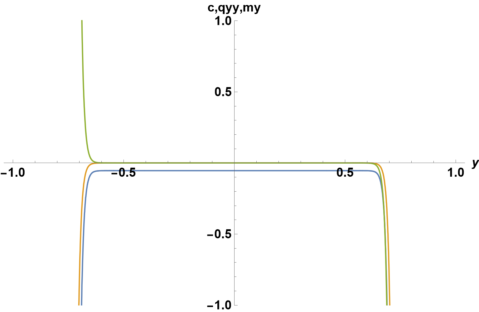
Plot[c[y] /. sol, {y, -1, 1}, PlotRange -> All]

NDSolve::bvluc: The equations derived from the boundary conditions are numerically ill-conditioned. The boundary conditions may not be sufficient to uniquely define a solution. If a solution is computed, it may match the boundary conditions poorly.

NDSolve::berr: The scaled boundary value residual error of 2.9891304910534367`*^10 indicates that the boundary values are not satisfied to specified tolerances. Returning the best solution found.

Is there something I am missing in here? Even varying the number of points does not seem to have any effect on the result.

Answer 1

Because this system of equations is linear with constant coefficients, it can be solves symbolically.

sol = DSolveValue[eqs, {c[y], qyy[y], my[y]}, {y, -1, 1}];

With

LeafCount@sol
(* 73666 *)

sol is too lengthy to reproduce here. It can, however, be plotted without difficulty. For instance,

Plot[Evaluate[sol /. {d -> .1, l -> .1}], {y, -1, 1}, PlotRange -> {-1, 1}, 
  ImageSize -> Large,  AxesLabel -> {y, "c,qyy,my"}, LabelStyle -> {15, Bold, Black}]

Values near the endpoints are exponentially large, literally.

sol /. {d -> .1, l -> .1, y -> -1}
(* {-3.60777*10^11, -1.18112*10^11, 4.46677*10^11} *)
sol /. {d -> .1, l -> .1, y -> 1}
(* {-4.12317*10^11, -1.18112*10^11, -4.98216*10^11} *)

It is understandable that NDSolve has progressively more difficulty solving these equations as d and l approach zero.