1
$\begingroup$

It's possible to implement some bounded interval using Findroot ?

I'm trying to solve this kind of equation:

EFO = e[0.150/hbarc, 0.300/hbarc]
troot[\[Eta]_] := 
 FindRoot[e[Tc[\[Tau], 0, 0, \[Eta]], Mc[\[Tau], 0, 0, \[Eta]]] - 
    EFO == 0, {\[Tau], tmin}]
tfo[\[Eta]_] := troot[\[Eta]][[1, 2]]

That gave me the solution, however the findroot try to solve on each possible Eta, can I give some boundary like, solve this equation between emin and emax ?

I tried to do it using NSolve, however Tc and Mc are interpolation variables coming from another code, so I guess I can't use it ?

e is a previous equation set analytically previously. I can put here the equation if needed:

dn0dTfull[T_] = g T^2 (m/T)^2 (3 BesselK[2,m/T] + m/T BesselK[1, m/T]);
e0full[T_] = T^2 dn0dTfull[T]; 
e[T_, \[Mu]_] = 4 Cosh[\[Mu]/T] e0full[T];

Here to experiment, I give tables of Tc and Mc:

    In[328]:= Table[
     Tc[t, 0, 0, \[Eta]], {t, tmin, tmax}, {\[Eta], emin, emax}]
    
    Out[328]= {{0.182292, 0.269708, 0.383436, 0.523777, 0.687455, 
      0.866924, 1.05039, 1.2228, 1.3677, 1.4698, 1.51759, 1.50549, 
      1.43494, 1.31408, 1.15622, 0.977434, 0.793908, 0.619567, 0.464566, 
      0.334698, 0.231697}, {0.0716525, 0.107187, 0.156508, 0.229516, 
      0.343474, 0.516587, 0.732682, 0.883657, 0.986054, 1.05251, 1.08255, 
      1.075, 1.0302, 0.949548, 0.831047, 0.649025, 0.43933, 0.291726, 
      0.196482, 0.134692, 0.0915409}, {0.0507062, 0.0757684, 0.111338, 
      0.165161, 0.250609, 0.381221, 0.56341, 0.755404, 0.868255, 0.931962,
       0.959483, 0.952628, 0.911084, 0.830745, 0.686618, 0.484546, 
      0.322895, 0.211689, 0.140663, 0.0955352, 0.0646638}, {0.0406486, 
      0.0606893, 0.0895268, 0.133691, 0.204502, 0.31325, 0.465137, 
      0.649319, 0.788629, 0.857957, 0.885968, 0.879072, 0.836034, 
      0.743793, 0.574322, 0.399305, 0.264661, 0.172186, 0.113522, 
      0.0766878, 0.0517963}, {0.0345122, 0.0515018, 0.0761779, 0.11427, 
      0.175759, 0.270539, 0.403, 0.566266, 0.719236, 0.800501, 0.830989, 
      0.823599, 0.775686, 0.665203, 0.498455, 0.345599, 0.228166, 
      0.147658, 0.0968363, 0.0651772, 0.043962}, {0.0302976, 0.0451988, 
      0.0669884, 0.10082, 0.155703, 0.240553, 0.359234, 0.50569, 0.654801,
       0.749498, 0.784292, 0.775988, 0.720338, 0.598097, 0.444744, 
      0.307807, 0.2026, 0.130594, 0.0853113, 0.0572655, 
      0.038588}, {0.0271878, 0.040552, 0.060195, 0.0908293, 0.14072, 
      0.21804, 0.326283, 0.459855, 0.598938, 0.70093, 0.741145, 0.731583, 
      0.667739, 0.544766, 0.404261, 0.279378, 0.183439, 0.117876, 
      0.0767692, 0.0514238, 0.0346258}, {0.0247795, 0.0369557, 0.0549257, 
      0.0830509, 0.129, 0.200356, 0.300337, 0.423706, 0.55287, 0.654777, 
      0.699501, 0.688678, 0.61995, 0.50225, 0.372359, 0.25701, 0.168411, 
      0.107946, 0.0701297, 0.046897, 0.0315589}, {0.0228483, 0.0340731, 
      0.0506942, 0.0767849, 0.119522, 0.186006, 0.279234, 0.394272, 
      0.514893, 0.612891, 0.659489, 0.647906, 0.578578, 0.467541, 
      0.346394, 0.23883, 0.156232, 0.0999284, 0.0647887, 0.0432647, 
      0.0291003}, {0.0212582, 0.0317005, 0.0472057, 0.0716055, 0.111661, 
      0.174069, 0.261646, 0.369716, 0.483089, 0.576205, 0.622387, 0.61068,
       0.543284, 0.438556, 0.324739, 0.223688, 0.146112, 0.093288, 
      0.0603791, 0.0402723, 0.0270763}, {0.0199216, 0.0297065, 0.04427, 
      0.0672368, 0.105012, 0.163946, 0.246704, 0.348834, 0.456001, 
      0.544392, 0.589068, 0.577625, 0.513025, 0.413894, 0.30633, 0.210831,
       0.137537, 0.0876774, 0.0566636, 0.0377556, 0.0253751}}

In[329]:= Table[
 Mc[t, 0, 0, \[Eta]], {t, tmin, tmax}, {\[Eta], emin, emax}]

Out[329]= {{1.52032, 1.52032, 1.52032, 1.52032, 1.52032, 1.52032, 
  1.52032, 1.52032, 1.52032, 1.52032, 1.52032, 1.52032, 1.52032, 
  1.52032, 1.52032, 1.52032, 1.52032, 1.52032, 1.52032, 1.52032, 
  1.52032}, {4.19032, 4.14321, 4.07089, 3.90298, 3.54315, 2.90001, 
  2.08765, 1.73248, 1.59702, 1.53413, 1.51001, 1.51586, 1.55363, 
  1.63881, 1.83013, 2.38222, 3.19601, 3.71638, 3.98759, 4.10636, 
  4.16302}, {4.6514, 4.61521, 4.55293, 4.4148, 4.12769, 3.62201, 
  2.85479, 2.06429, 1.7461, 1.62553, 1.583, 1.59314, 1.66132, 1.83529,
   2.3274, 3.1931, 3.85424, 4.26516, 4.48371, 4.58298, 
  4.63135}, {4.86377, 4.83399, 4.77925, 4.66, 4.4148, 3.98492, 
  3.33344, 2.50136, 1.93724, 1.73663, 1.67175, 1.68695, 1.79358, 
  2.09935, 2.84226, 3.62126, 4.18217, 4.532, 4.71927, 4.80544, 
  4.84737}, {4.99029, 4.96462, 4.91548, 4.80944, 4.59256, 4.21295, 
  3.63835, 2.88702, 2.18107, 1.8699, 1.77523, 1.79703, 1.95623, 
  2.42261, 3.20363, 3.8921, 4.38709, 4.69615, 4.86205, 4.93887, 
  4.97608}, {5.07579, 5.05301, 5.0082, 4.91205, 4.716, 4.37302, 
  3.85404, 3.17439, 2.45686, 2.03096, 1.89696, 1.92748, 2.1545, 
  2.73013, 3.46155, 4.08317, 4.53036, 4.8096, 4.9597, 5.02946, 
  5.0631}, {5.13815, 5.11753, 5.07617, 4.98778, 4.80788, 4.49318, 
  4.01694, 3.39337, 2.71474, 2.21975, 2.04045, 2.08161, 2.37713, 
  2.98167, 3.65689, 4.22718, 4.63755, 4.89376, 5.03156, 5.09574, 
  5.12658}, {5.18601, 5.16707, 5.12856, 5.04645, 4.87955, 4.58754, 
  4.14552, 3.56686, 2.93259, 2.42194, 2.20472, 2.25626, 2.59588, 
  3.18408, 3.8114, 4.34066, 4.72152, 4.95922, 5.08709, 5.14675, 
  5.17532}, {5.22411, 5.20654, 5.17041, 5.09353, 4.93738, 4.66411, 
  4.25031, 3.70863, 3.11382, 2.61621, 2.38005, 2.43832, 2.79125, 
  3.35016, 3.93753, 4.43299, 4.78951, 5.01191, 5.13156, 5.18745, 
  5.21413}, {5.2553, 5.23885, 5.20476, 5.13231, 4.98524, 4.72779, 
  4.33779, 3.82726, 3.26633, 2.79057, 2.55194, 2.6124, 2.96001, 
  3.48935, 4.04299, 4.50998, 4.84595, 5.05544, 5.16814, 5.22082, 
  5.24592}, {5.28138, 5.2659, 5.23356, 5.16493, 5.02567, 4.7818, 
  4.41221, 3.92839, 3.39669, 2.94339, 2.71048, 2.77029, 3.10559, 
  3.60815, 4.13283, 4.5754, 4.89374, 5.09214, 5.19887, 5.24878, 
  5.27251}}

Here the values of some settings

tmin = 0.25;
tmax = 10.25;
emin = -10.3;
emax = 10.3;
hbarc = 0.197326938; 
GeV = 1/hbarc;
m = 1.116 GeV;
g = 1/(2 Pi^2);

Thank you for the answers

$\endgroup$
3
  • 1
    $\begingroup$ Without the definitions for Tc and Mc there is no way for us to experiment. Also if you are looking to work on a bounded interval for η, please specify the interval of interest. $\endgroup$
    – Bob Hanlon
    Commented Aug 18, 2021 at 11:24
  • $\begingroup$ thanks for the answer, I added the tables because I can't give directly the interpolated functions $\endgroup$
    – G. Sophys
    Commented Aug 18, 2021 at 12:23
  • $\begingroup$ Also, what are the values for m and g? $\endgroup$
    – Bob Hanlon
    Commented Aug 18, 2021 at 13:25

1 Answer 1

0
$\begingroup$

EDIT: Revised for addition of GeV = 1/hbarc

Clear["Global`*"]

dn0dTfull[T_] = g T^2 (m/T)^2 (3 BesselK[2, m/T] + m/T BesselK[1, m/T]);
e0full[T_] = T^2 dn0dTfull[T];
e[T_, μ_] = 4 Cosh[μ/T] e0full[T];

EFO = e[(15/100)/hbarc, (3/10)/hbarc] // Simplify;

tmin = 0.25;
tmax = 10.25;
emin = -10.3;
emax = 9.7;(* Your Table only goes to 9.7 rather than 10.3 *)

hbarc = 0.197326938;
GeV = 1/hbarc;
m = 1.116 GeV;
g = 1/(2 Pi^2);

Your tabular data:

dataTc = {{0.182292, 0.269708, 0.383436, 0.523777, 0.687455, 0.866924, 
    1.05039, 1.2228, 1.3677, 1.4698, 1.51759, 1.50549, 1.43494, 1.31408, 
    1.15622, 0.977434, 0.793908, 0.619567, 0.464566, 0.334698, 
    0.231697}, {0.0716525, 0.107187, 0.156508, 0.229516, 0.343474, 0.516587, 
    0.732682, 0.883657, 0.986054, 1.05251, 1.08255, 1.075, 1.0302, 0.949548, 
    0.831047, 0.649025, 0.43933, 0.291726, 0.196482, 0.134692, 
    0.0915409}, {0.0507062, 0.0757684, 0.111338, 0.165161, 0.250609, 0.381221,
     0.56341, 0.755404, 0.868255, 0.931962, 0.959483, 0.952628, 0.911084, 
    0.830745, 0.686618, 0.484546, 0.322895, 0.211689, 0.140663, 0.0955352, 
    0.0646638}, {0.0406486, 0.0606893, 0.0895268, 0.133691, 0.204502, 0.31325,
     0.465137, 0.649319, 0.788629, 0.857957, 0.885968, 0.879072, 0.836034, 
    0.743793, 0.574322, 0.399305, 0.264661, 0.172186, 0.113522, 0.0766878, 
    0.0517963}, {0.0345122, 0.0515018, 0.0761779, 0.11427, 0.175759, 0.270539,
     0.403, 0.566266, 0.719236, 0.800501, 0.830989, 0.823599, 0.775686, 
    0.665203, 0.498455, 0.345599, 0.228166, 0.147658, 0.0968363, 0.0651772, 
    0.043962}, {0.0302976, 0.0451988, 0.0669884, 0.10082, 0.155703, 0.240553, 
    0.359234, 0.50569, 0.654801, 0.749498, 0.784292, 0.775988, 0.720338, 
    0.598097, 0.444744, 0.307807, 0.2026, 0.130594, 0.0853113, 0.0572655, 
    0.038588}, {0.0271878, 0.040552, 0.060195, 0.0908293, 0.14072, 0.21804, 
    0.326283, 0.459855, 0.598938, 0.70093, 0.741145, 0.731583, 0.667739, 
    0.544766, 0.404261, 0.279378, 0.183439, 0.117876, 0.0767692, 0.0514238, 
    0.0346258}, {0.0247795, 0.0369557, 0.0549257, 0.0830509, 0.129, 0.200356, 
    0.300337, 0.423706, 0.55287, 0.654777, 0.699501, 0.688678, 0.61995, 
    0.50225, 0.372359, 0.25701, 0.168411, 0.107946, 0.0701297, 0.046897, 
    0.0315589}, {0.0228483, 0.0340731, 0.0506942, 0.0767849, 0.119522, 
    0.186006, 0.279234, 0.394272, 0.514893, 0.612891, 0.659489, 0.647906, 
    0.578578, 0.467541, 0.346394, 0.23883, 0.156232, 0.0999284, 0.0647887, 
    0.0432647, 0.0291003}, {0.0212582, 0.0317005, 0.0472057, 0.0716055, 
    0.111661, 0.174069, 0.261646, 0.369716, 0.483089, 0.576205, 0.622387, 
    0.61068, 0.543284, 0.438556, 0.324739, 0.223688, 0.146112, 0.093288, 
    0.0603791, 0.0402723, 0.0270763}, {0.0199216, 0.0297065, 0.04427, 
    0.0672368, 0.105012, 0.163946, 0.246704, 0.348834, 0.456001, 0.544392, 
    0.589068, 0.577625, 0.513025, 0.413894, 0.30633, 0.210831, 0.137537, 
    0.0876774, 0.0566636, 0.0377556, 0.0253751}};

To recreate the InterpolatingFunction from your Table values

tc = Interpolation[
   Transpose[{Flatten[
      Table[{t, η}, {t, tmin, tmax}, {η, emin, emax}], 1], 
     dataTc // Flatten}]];

Tc[t_, 0, 0, η_] := tc[t, η];

Verifying,

Table[Tc[t, 0, 0, η], {t, tmin, tmax}, {η, emin, emax}] == dataTc

(* True *)

Similarly, for your other Table

dataMc = {{1.52032, 1.52032, 1.52032, 1.52032, 1.52032, 1.52032, 1.52032, 
    1.52032, 1.52032, 1.52032, 1.52032, 1.52032, 1.52032, 1.52032, 1.52032, 
    1.52032, 1.52032, 1.52032, 1.52032, 1.52032, 1.52032}, {4.19032, 4.14321, 
    4.07089, 3.90298, 3.54315, 2.90001, 2.08765, 1.73248, 1.59702, 1.53413, 
    1.51001, 1.51586, 1.55363, 1.63881, 1.83013, 2.38222, 3.19601, 3.71638, 
    3.98759, 4.10636, 4.16302}, {4.6514, 4.61521, 4.55293, 4.4148, 4.12769, 
    3.62201, 2.85479, 2.06429, 1.7461, 1.62553, 1.583, 1.59314, 1.66132, 
    1.83529, 2.3274, 3.1931, 3.85424, 4.26516, 4.48371, 4.58298, 
    4.63135}, {4.86377, 4.83399, 4.77925, 4.66, 4.4148, 3.98492, 3.33344, 
    2.50136, 1.93724, 1.73663, 1.67175, 1.68695, 1.79358, 2.09935, 2.84226, 
    3.62126, 4.18217, 4.532, 4.71927, 4.80544, 4.84737}, {4.99029, 4.96462, 
    4.91548, 4.80944, 4.59256, 4.21295, 3.63835, 2.88702, 2.18107, 1.8699, 
    1.77523, 1.79703, 1.95623, 2.42261, 3.20363, 3.8921, 4.38709, 4.69615, 
    4.86205, 4.93887, 4.97608}, {5.07579, 5.05301, 5.0082, 4.91205, 4.716, 
    4.37302, 3.85404, 3.17439, 2.45686, 2.03096, 1.89696, 1.92748, 2.1545, 
    2.73013, 3.46155, 4.08317, 4.53036, 4.8096, 4.9597, 5.02946, 
    5.0631}, {5.13815, 5.11753, 5.07617, 4.98778, 4.80788, 4.49318, 4.01694, 
    3.39337, 2.71474, 2.21975, 2.04045, 2.08161, 2.37713, 2.98167, 3.65689, 
    4.22718, 4.63755, 4.89376, 5.03156, 5.09574, 5.12658}, {5.18601, 5.16707, 
    5.12856, 5.04645, 4.87955, 4.58754, 4.14552, 3.56686, 2.93259, 2.42194, 
    2.20472, 2.25626, 2.59588, 3.18408, 3.8114, 4.34066, 4.72152, 4.95922, 
    5.08709, 5.14675, 5.17532}, {5.22411, 5.20654, 5.17041, 5.09353, 4.93738, 
    4.66411, 4.25031, 3.70863, 3.11382, 2.61621, 2.38005, 2.43832, 2.79125, 
    3.35016, 3.93753, 4.43299, 4.78951, 5.01191, 5.13156, 5.18745, 
    5.21413}, {5.2553, 5.23885, 5.20476, 5.13231, 4.98524, 4.72779, 4.33779, 
    3.82726, 3.26633, 2.79057, 2.55194, 2.6124, 2.96001, 3.48935, 4.04299, 
    4.50998, 4.84595, 5.05544, 5.16814, 5.22082, 5.24592}, {5.28138, 5.2659, 
    5.23356, 5.16493, 5.02567, 4.7818, 4.41221, 3.92839, 3.39669, 2.94339, 
    2.71048, 2.77029, 3.10559, 3.60815, 4.13283, 4.5754, 4.89374, 5.09214, 
    5.19887, 5.24878, 5.27251}};

Recreating the InterpolatingFunction

mc = Interpolation[
   Transpose[{Flatten[
      Table[{t, η}, {t, tmin, tmax}, {η, emin, emax}], 1], 
     dataMc // Flatten}]];

Mc[t_, 0, 0, η_] := mc[t, η];

Verifying,

Table[Mc[t, 0, 0, η], {t, tmin, tmax}, {η, emin, emax}] == dataMc

(* True *)

Plotting,

f[τ_?NumericQ, η_?NumericQ] := 
 e[Tc[τ, 0, 0, η], Mc[τ, 0, 0, η]] - EFO

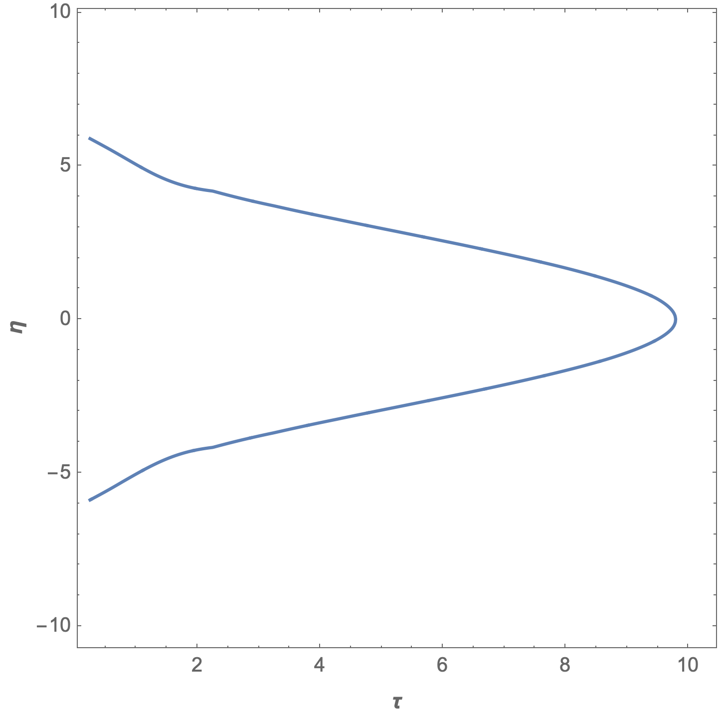
ContourPlot[f[τ, η] == 0,
 {τ, tmin, tmax}, {η, emin, emax},
 FrameLabel -> (Style[#, 12, Bold] & /@ {τ, η}),
 PlotPoints -> 100,
 MaxRecursion -> 3]

enter image description here

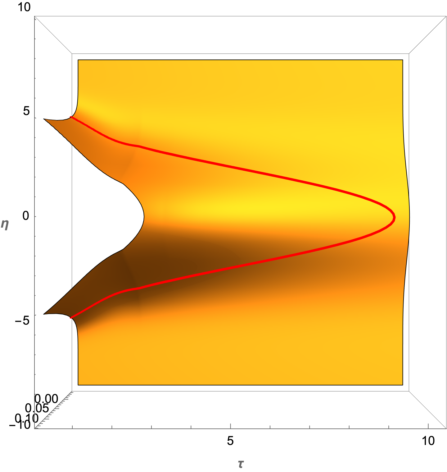
Plot3D[f[τ, η], {τ, tmin, tmax}, {η, emin, emax},
 AxesLabel -> (Style[#, 12, Bold] & /@ {τ, η}),
 ClippingStyle -> None,
 PlotPoints -> 100,
 MaxRecursion -> 2,
 MeshFunctions -> (#3 &),
 Mesh -> {{0}},
 MeshStyle -> {Red, Thick},
 ViewPoint -> Above]

enter image description here

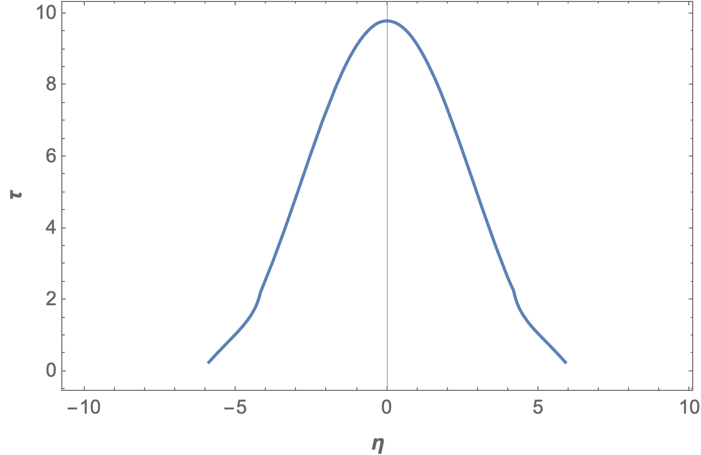
troot[η_?NumericQ] := 
 Check[τ /. 
   FindRoot[f[τ, η] == 0, {τ, tmin, tmin, tmax}], $Failed]

Plot[troot[η], {η, emin, emax},
  Frame -> True,
  FrameLabel -> (Style[#, 12, Bold] & /@
     {η, τ})] // Quiet

enter image description here

$\endgroup$
3
  • $\begingroup$ firstly, thank you for the answer, in this troot[η_?NumericQ] := Check[τ /. FindRoot[f[τ, η] == 0, {τ, tmin, tmin, tmax}], $Failed] as I understand, you have the bounded interval for t, but there is an implicit interval for eta ? $\endgroup$
    – G. Sophys
    Commented Aug 19, 2021 at 9:59
  • $\begingroup$ There is nothing implicit about eta, it is the explicit numeric argument to troot. The eta range iterator in the various plotting functions define its range. $\endgroup$
    – Bob Hanlon
    Commented Aug 19, 2021 at 12:15
  • $\begingroup$ Okay, consequently he calculate each time the Findroot for this particular point of eta in the function ? Great, it's perfectly what I needed, thank you ! $\endgroup$
    – G. Sophys
    Commented Aug 19, 2021 at 13:09

Your Answer

By clicking “Post Your Answer”, you agree to our terms of service and acknowledge you have read our privacy policy.

Not the answer you're looking for? Browse other questions tagged or ask your own question.