Mathematica integrates too well using the "code" I wrote

Question

I am trying to make Mathematica do the following: Split up the interval [0,1] into $n$ equal intervals. Then on each interval apply the Gaussian Quadrature for 2 points.

I tried to use the method from mky question here:Using Composite Newton-Cotes integration rules in Mathematica

But the results I am getting are way too accurate.

Here is the code:

n = 1;                                                                                                            
NIntegrate[Sin[x]/x, Evaluate@Flatten@{x, Subdivide[0., 1., n]}, 
 Method -> {"GaussBerntsenEspelidRule", "Points" -> 2}, 
 MaxRecursion -> 0]

So what this should be doing is just do the Gaussian Quadrature with 2 points on $[0,1]$ but I am getting the answer with at least $10^{-5}$ accuracy which should not be happening. What did I do wrong?

Answer 1

You're just lucky (as far as getting low error):

{abs, wts, err} = 
 NIntegrate`GaussBerntsenEspelidRuleData[2, MachinePrecision]

(*
  {{0.0469101, 0.230765, 0.5, 0.769235, 0.95309},
   {0.118463, 0.239314, 0.284444, 0.239314, 0.118463},
   {0.155257, -0.439701, 0.568889, -0.439701, 0.155257}}
*)

(Sin[x]/x /. x -> abs).wts
(Sin[x]/x /. x -> abs).err

(*
  0.946083       <-- integral estimate
  0.0000639286   <-- estimated error bound
*)

(Sin[x]/x /. x -> abs).wts - Integrate[Sin[x]/x, {x, 0, 1}]

(*
  3.31957*10^-14  <-- actual error (less than the bound)
*)

The above code reproduces the NIntegrate result:

(Sin[x]/x /. x -> abs).wts -
 NIntegrate[Sin[x]/x, Evaluate@Flatten@{x, Subdivide[0., 1., nn]}, 
  Method -> {"GaussBerntsenEspelidRule", "Points" -> 2}, 
  MaxRecursion -> 0]

(*
  0.
*)

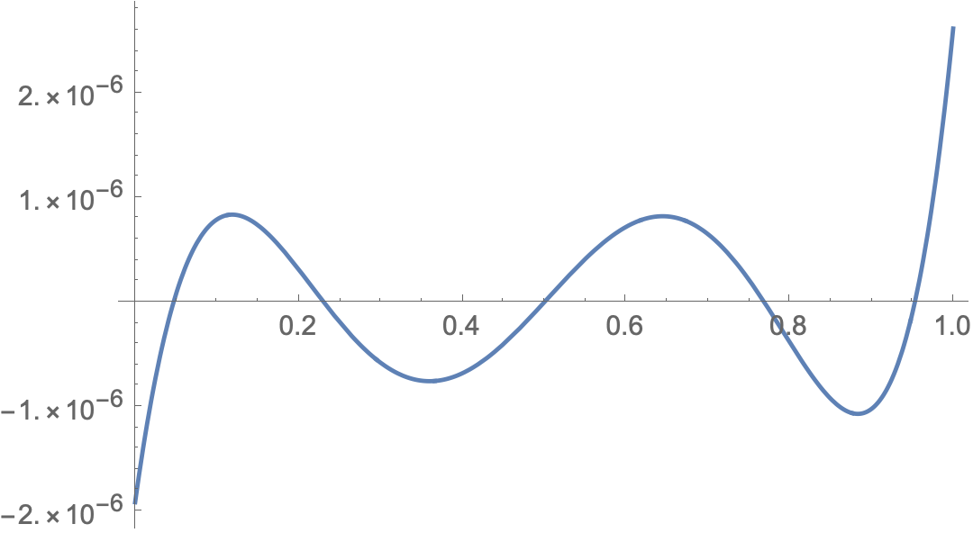
Why are we lucky in this case? The error is equal to the integral of the difference of the function and the interpolating polynomial through abscissae abs, which roughly has the same area above and below the x axis:

Plot[
 InterpolatingPolynomial[Transpose@{abs, (Sin[x]/x /. x -> abs)}, x] -
  Sin[x]/x // Evaluate,
 {x, 0, 1}]