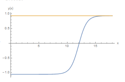
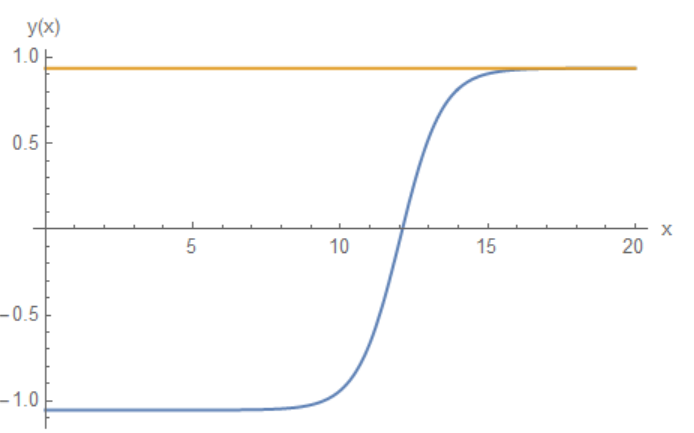
We can play with initial value ys to get solution at xm=20. For this we should increase precision of roots as follows
a = 23/100;
V[y_] := (1/4) (y^2 - 1)^2 + a (y - 1)/(2);
ode = y''[x] + (3 y'[x])/x == V'[y[x]];
extrema =
 Block[{y},
  Rationalize[
   y /. NSolve[D[V[y], y] == 0, y, Reals, WorkingPrecision -> 50],
   10^-49]]
Also we need to increase precision of solution
xs = 10^-8; xm = 20;
s = ParametricNDSolve[{ode, y'[xs] == 0, y[xm] == extrema[[3]]},
   y, {x, xs, xm}, {ys},
   Method -> {"Shooting",
     "StartingInitialConditions" -> {y[xs] == ys, y'[xs] == 0}},
   WorkingPrecision -> 30];
Finally we can plot desired solution playing with ys (this is really trick!)
f = y[extrema[[1]] + 2 10^-6 + 10^-7] /.
  s;(*choosing the optimal value of ys to get the correct \
solution*)f[xs]
Plot[{f[x], extrema[[3]]}, {x, xs, xm}, AxesLabel -> {"x", "y(x)"},
 PlotRange -> All]

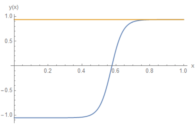
Now we use the wavelets collocation method to get numerical solution for large and small intervals with xm=L. First, we map interval $(0,L)$ to $(0,1)$ using substitution $x\rightarrow L x$. Second, we use numerical solution at $L=21$ as initial guess to generate sequence of numerical solutions. Here we put xm=1 since we map interval to $(0,1)$:
a = 23/100; L = 21;
V[y_] := (1/4) (y^2 - 1)^2 + a (y - 1)/(2);
ode = y''[x] + (3 y'[x])/x == L^2 V'[y[x]];
extrema =
  Block[{y},
   Rationalize[
    y /. NSolve[D[V[y], y] == 0, y, Reals, WorkingPrecision -> 120],
    10^-119]];


xs = 10^-8; xm = 1;
s = ParametricNDSolve[{ode, y'[xs] == 0, y[xm] == extrema[[3]],
    WhenEvent[y'[x] < 0, {xmax = x, "StopIntegration"}]},
   y, {x, xs, xm}, {ys},
   Method -> {"Shooting",
     "StartingInitialConditions" -> {y[xs] == ys, y'[xs] == 0}},
   WorkingPrecision -> 30];


pp = -(149643685212592894317733320513154810629526671825404636079551673\
152787/142087466431502699344020314203802217303945506305721123722555300\
000000); f =
 y[pp] /. s;(*choosing the optimal value of ys to get the correct \
solution*)
Plot[{f[x], extrema[[3]]}, {x, xs, xm}, AxesLabel -> {"x", "y(x)"},
 PlotRange -> All]
Numerical solution at $L=21$

With this code we calculate initial guess for Harr wavelets method:
 J = 5; M = 2^J; dx = 1/(2*M); h1[x_] := Piecewise[{{1, 0 <= x <= 1}, {0, True}}];
  p1[x_, n_] := (1/n!)*x^n;
h[x_, k_, m_] := Piecewise[{{1, Inequality[k/m, LessEqual, x, Less, (1 + 2*k)/(2*m)]},
    {-1, Inequality[(1 + 2*k)/(2*m), LessEqual, x, Less, (1 + k)/m]}}, 0]
p[x_, k_, m_, n_] := Piecewise[{{0, x < k/m}, {(-(k/m) + x)^n/n!, Inequality[k/m, LessEqual, x,
      Less, (1 + 2*k)/(2*m)]}, {((-(k/m) + x)^n - 2*(-((1 + 2*k)/(2*m)) + x)^n)/n!,
     (1 + 2*k)/(2*m) <= x <= (1 + k)/m},
    {((-(k/m) + x)^n + (-((1 + k)/m) + x)^n - 2*(-((1 + 2*k)/(2*m)) + x)^n)/n!, x > (1 + k)/m}}, 0]
xl = Table[l*dx, {l, 0, 2*M}]; xcol = Table[(xl[[l - 1]] + xl[[l]])/2, {l, 2, 2*M + 1}];
f2[x_] := Sum[af[i, j]*h[x, i, 2^j], {j, 0, J, 1}, {i, 0, 2^j - 1, 1}] + a0*h1[x];
  f1[x_] := Sum[af[i, j]*p[x, i, 2^j, 1], {j, 0, J, 1}, {i, 0, 2^j - 1, 1}] + a0*p1[x, 1] + f10;
  f0[x_] := Sum[af[i, j]*p[x, i, 2^j, 2], {j, 0, J, 1}, {i, 0, 2^j - 1, 1}] + a0*p1[x, 2] + f10*x +
    f00;

bc = {f1[0] == 0, f0[1] == extrema[[3]]}; var =
 Flatten[Table[af[i, j], {j, 0, J, 1}, {i, 0, 2^j - 1, 1}]];
varM = Join[{a0, f10, f00}, var]; eq = Table[f0[x] == f[x], {x, xcol}];
eqM = Join[eq, bc];

sol0 = NSolve[eqM, varM];
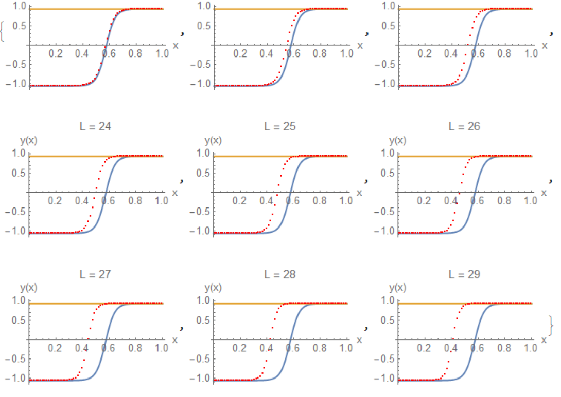
Finally we compute sequence of numerical solutions for $21\le L\le 29$:
sol[0] = sol0[[1]]; L = 20; Do[L = L + 1;
 eqn[x_] := f2[x] + (3 f1[x])/x - L^2 V'[f0[x]];
 eq1 = Table[eqn[x] == 0, {x, xcol}];
 eqM1 = Join[eq1, bc];
 sol[j] = FindRoot[eqM1,
   Table[{varM[[i]], Last[sol[j - 1][[i]]]}, {i, Length[varM]}]];
 lst1 = Table[{x, Evaluate[f0[x] /. sol[j]]}, {x, xcol}];
 plot[j] =
  Show[Plot[{f[x], extrema[[3]]}, {x, xs, xm},
    AxesLabel -> {"x", "y(x)"}, PlotRange -> All,
    PlotLabel -> Row[{"L = ", L}]],
   ListPlot[lst1, PlotStyle -> Red]];, {j, 1, 9}]
Visualisation of numerical solutions (red points) together with initial guess (blue line)
Table[plot[j], {j, 9}]

Final remarks: to get solution at $L>29$ we need to put in do loop L=L+1/2. For example,
sol[0] = sol[9]; L = 29; Do[L = L + 1/2;
 eqn[x_] := f2[x] + (3 f1[x])/x - L^2 V'[f0[x]];
 eq1 = Table[eqn[x] == 0, {x, xcol}];
 eqM1 = Join[eq1, bc];
 sol[j] = FindRoot[eqM1,
   Table[{varM[[i]], Last[sol[j - 1][[i]]]}, {i, Length[varM]}]];
 lst1 = Table[{x, Evaluate[f0[x] /. sol[j]]}, {x, xcol}];
 plot[j] =
  Show[Plot[{f[x], extrema[[3]]}, {x, xs, xm},
    AxesLabel -> {"x", "y(x)"}, PlotRange -> All,
    PlotLabel -> Row[{"L = ", L // N}]],
   ListPlot[lst1, PlotStyle -> Red]];, {j, 1, 10}]

Table[plot[j], {j, 10}]

For $L<21$ we use
sol[0] = sol0[[1]]; L = 21; Do[L = L - 1/4;
 eqn[x_] := f2[x] + (3 f1[x])/x - L^2 V'[f0[x]];
 eq1 = Table[eqn[x] == 0, {x, xcol}];
 eqM1 = Join[eq1, bc];
 sol[j] = FindRoot[eqM1,
   Table[{varM[[i]], Last[sol[j - 1][[i]]]}, {i, Length[varM]}]];
 lst1 = Table[{x, Evaluate[f0[x] /. sol[j]]}, {x, xcol}];
 plot[j] =
  Show[Plot[{f[x], extrema[[3]]}, {x, xs, xm},
    AxesLabel -> {"x", "y(x)"}, PlotRange -> All,
    PlotLabel -> Row[{"L = ", L // N}]],
   ListPlot[lst1, PlotStyle -> Red]];, {j, 1, 10}]


