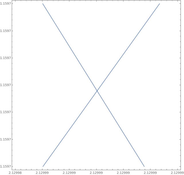
Simplest plotting solution
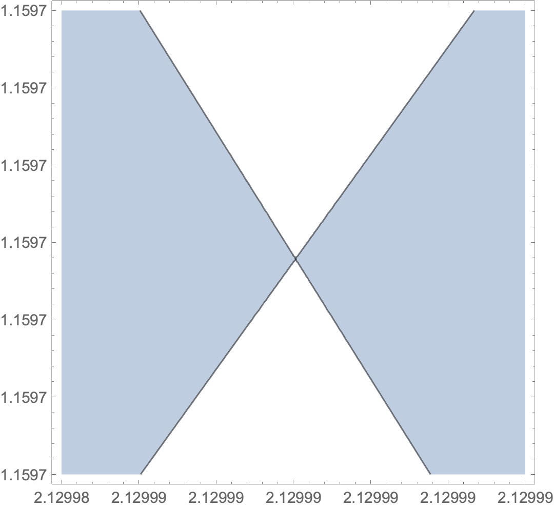
ContourPlot[f,
 {y, Rationalize[2.1299849, 0],  Rationalize[2.1299855, 0]},
 {x, Rationalize[1.15970110, 0], Rationalize[1.15970113, 0]},
 ContourShading ->
  {RGBColor[0.368417, 0.506779, 0.709798, 0.4], None},
 Contours -> {{0}},
 PlotPoints -> 25, WorkingPrecision -> 32,
 Method -> {"TransparentPolygonMesh" -> True}
 ]

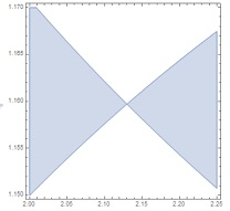
But plots are not always very convincing, being designed to give only a rough idea of what is going on.
Analytic solution
As I showed in this answer to a similar question, we can analytically show there's a node:
jac = D[f, {{x, y}}];
cpsol = FindRoot[jac == {0, 0}, {{x, 1.15}, {y, 2.13}},
   WorkingPrecision -> 50];
cpt = {x, y} /. cpsol
f /. cpsol      (* shows cpt is on curve *)
f /. N[cpsol]   (* show numerical noise at cpt is substantial *)
(*
  {1.1597011139328870007473930523093558428367204499142,
   2.1299852028277681162523681416937176426970454505325}
  0.*10^-36
  0.0119859
*)
Taming RegionPlot
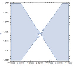
RegionPlot has been evolving since the introduction of Region functionality. RegionPlot seems to use this functionality to generate the plot, and it ignores the WorkingPrecision option, which is evident from the numerical noise. I believe the region functionality is based on the FEM functionality, which is available only in machine precision. (Similarly, the option MaxRecursion seems defunct.)
Here is a way to sieze control of the working precision:
ClearAll[fff];
fff[x0_Real, y0_Real] :=
  Block[{x = SetPrecision[x0, Infinity],
    y = SetPrecision[y0, Infinity]},
   N[
    1024 (1 - (9 x^2)/4)^2 Cosh[(π x)/
        3]^2 Sinh[π x]^2 (8 (16 - 216 x^2 +
          81 x^4 + (4 + 9 x^2)^2 Cosh[(2 π x)/
             3]) Sinh[π x]^2 -
       1/256 ((4 + 9 x^2)^2 Sinh[x (2 π - y)] +
           2 (64 - 144 x^2 + (4 + 9 x^2)^2 Cosh[(2 π x)/3]) Sinh[
             x y] - 9 (4 - 3 x^2)^2 Sinh[x (2 π + y)])^2),
    $MachinePrecision]
   ];

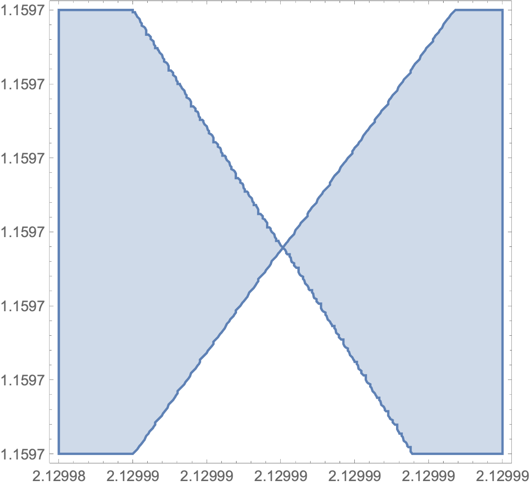
RegionPlot[
 fff[x, y] < 0,
 {y, Rationalize[2.1299849, 0],  Rationalize[2.1299855, 0]},
 {x, Rationalize[1.15970110, 0], Rationalize[1.15970113, 0]},
 PlotPoints -> 100]

But one swallow does not a summer make.

