1-D prey-predator system with diffusion and time-dependent parameters in Mathematica 12

Question

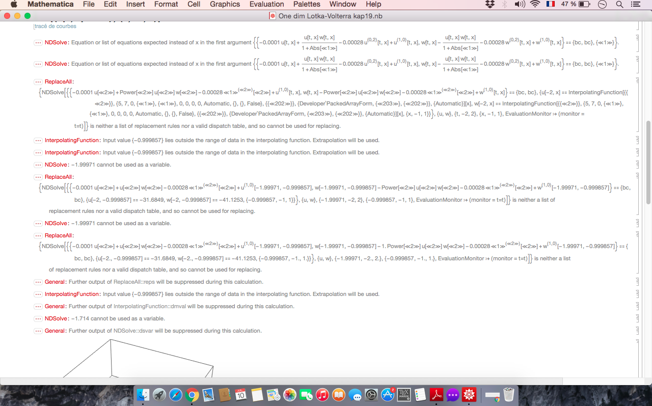
Please you find attached a Mathematica program for the existence of almost periodic solutions for a class of Lotka-Volterra prey-predators systems with diffusion and time-dependent parameters in Mathematica 12. The program is finished but there are some problems, I don't know exactly where. I have changed a lot but the same problem. I will be grateful if someone gives an idea about it. Thank you in advance.

pts = 100;
tmax = 50;
(*length of square*)L = 1;(*Time integration*)T = 2;(*Diffusion \
parameter for the prey*)d1 = 0.00028;(*Diffusion parameter for the \
predator*)d2 = 0.00028;(*Fertility parameter for the prey*)a = \
0.0001;(*Mortality parameter of the prey in the presence of \
predator*)b = 0.1;(*Fertility parameter of the predator*)c1 = \
1;(*Fertility parameter of the predator in the presence of the \
prey*)c2 = 1;

(*system of nonlinear PDEs*)

pde = {D[u[t, x], t] - d1*(2 + Cos[t]) *D[u[t, x], x, x] + 
    a*(2 + Cos[1/(3 + Cos[t] + Cos[Sqrt[2] t])])* u[t, x] - 
    c1*(3 + Sin[t] + Sin[Sqrt[2] t])* u[t, x]*
     w[t, x]/(1 + Abs[D[x[t, x], x]]),
   D[w[t, x], t] - d2*(2 + Cos[t])* D[w[t, x], x, x] - 
    b* (2 + Sin[1/(3 + Sin[t/4] + Sin[Sqrt[2] t])])* w[t, x] + 
    c2*Piecewise[{{1 + Cos[t], t < 0}, {1 + Sin[t], t >= 0}}, 0]* 
     u[t, x]*w[t, x]/(1 + Abs[D[u[t, x], x]])};

u0 = Interpolation[
  Flatten[Table[{x, RandomReal[]}, {x, -L, L, 2/pts}, 1]]]; w0 = 
 Interpolation[
  Flatten[Table[{x, RandomReal[]}, {x, -L, L, 2/pts}, 1]]];
reg = Rectangle[{-L, -L}, {L, L}];

ic = {u[-T, x] == u0[x], w[-T, x] == w0[x], {x, -L, L}};
(*Newman boundary condition*)
(*bc=NeumannValue[0,True];*)
\
(*Dirichlet boundary condition*)

bc = {u[t, L] == 0, u[t, -L] = 0, w[t, L] == 0, w[t, -L] == 0};
eqns = {pde == {bc, bc}, ic};
sol = NDSolve[eqns, {u, w}, {t, -T, T}, {x, -L, L}];
(Monitor[sol = 
    NDSolve[eqns, {u, w}, {t, -T, T}, {x, -L, L}, 
     EvaluationMonitor :> (monitor = Row[{"t=", t}])], monitor]);
(*Table[DensityPlot[Evaluate[u[t,x,y]/.First[sol]],{x,-L,L},{y,-L,L},\
ColorFunction\[Rule]Hue,PlotLabel\[Rule]Row[{"t=",t}],Frame\[Rule]\
False,PlotRange\[Rule]All],{t,0.05,.1,.02}]*)
Plot3D[
 Evaluate[u[t, x] /. sol], {t, -T, T}, {x, -L, L}, PlotRange -> All]
Plot[{u[t, 0] /. sol}, {t, -T, T}]

Answer 1

After minor corrections and typo removing's we have stable result with some options:

pts = 10; h = 1/pts;
tmax = 50;
(*length of square*)L = 1;(*Time integration*)T = 2;(*Diffusion \
parameter for the prey*)d1 = 0.00028;(*Diffusion parameter for the \
predator*)d2 = 0.00028;(*Fertility parameter for the prey*)a = \
0.0001;(*Mortality parameter of the prey in the presence of \
predator*)b = 0.1;(*Fertility parameter of the predator*)c1 = \
1;(*Fertility parameter of the predator in the presence of the \
prey*)c2 = 1;

(*system of nonlinear PDEs*)
f[t_] := Piecewise[{{1 + Cos[t], t < 0}, {1 + Sin[t], t >= 0}, {0, 
     True}}];
pde = {D[u[t, x], t] - d1*(2 + Cos[t])*D[u[t, x], x, x] + 
     a*(2 + Cos[1/(3 + Cos[t] + Cos[Sqrt[2] t])])*u[t, x] - 
     If[t > 10^-4, 
      c1*(3 + Sin[t] + Sin[Sqrt[2] t])*u[t, x]*
       w[t, x]/(1 + Evaluate[Abs[Derivative[0, 1][u][t, x]]]), 0] == 
    0, D[w[t, x], t] - d2*(2 + Cos[t])*D[w[t, x], x, x] - 
     b*(2 + Sin[1/(3 + Sin[t/4] + Sin[Sqrt[2] t])])*w[t, x] + 
     If[t > 10^-4, 
      c2*f[t]*u[t, x]*
       w[t, x]/(1 + Evaluate[Abs[Derivative[0, 1][u][t, x]]]), 0] == 
    0};
SeedRandom[1234];
u0 = Interpolation[
  Join[{{-L, 0}}, 
   Table[{x, RandomReal[]}, {x, -L + h, L - h, h}], {{L, 0}}], 
  InterpolationOrder -> 4]; w0 = 
 Interpolation[
  Join[{{-L, 0}}, 
   Table[{x, RandomReal[]}, {x, -L + h, L - h, h}], {{L, 0}}], 
  InterpolationOrder -> 4];


ic = {u[-T, x] == u0[x], w[-T, x] == w0[x]/10};
bc = {u[t, L] == 0, u[t, -L] == 0, w[t, L] == 0, w[t, -L] == 0};
eqns = Flatten[{pde, bc, ic}];


sol = NDSolve[eqns, {u, w}, {t, -T, T}, {x, -L, L}, 
   Method -> {"IndexReduction" -> Automatic, 
     "EquationSimplification" -> "Residual", 
     "PDEDiscretization" -> {"MethodOfLines", 
       "SpatialDiscretization" -> {"TensorProductGrid", 
         "MinPoints" -> 137, "MaxPoints" -> 137, 
         "DifferenceOrder" -> "Pseudospectral"}}}];


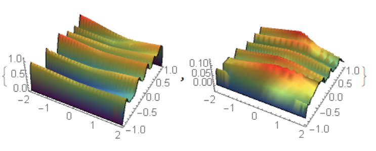
{Plot3D[Evaluate[u[t, x] /. sol], {t, -T, T}, {x, -L, L}, 
  PlotRange -> All, Mesh -> None, ColorFunction -> "Rainbow", 
  Boxed -> False], 
 Plot3D[Evaluate[w[t, x] /. sol], {t, -T, T}, {x, -L, L}, 
  PlotRange -> All, Mesh -> None, ColorFunction -> "Rainbow", 
  Boxed -> False]}