1
$\begingroup$

I have a Hamiltonian (Z) in matrix form, I solved it for time independent random real numbers, now want to introduce time dependent in such a way at any time the random real numbers change between the range {-Sqrt[3sigma2], Sqrt[3sigma2]}, here is my code

Nmax = 100; (*Number of sites*)

tini = 0; (*initial time*)

tmax = 200; (*maximal time*)

\[Sigma]2 = 0.1; (*Variance*)

n0 = 50; (*initial condition*)

ra = 1; (*coupling range*)

\[Psi]ini = Table[KroneckerDelta[n0 - i], {i, 1, Nmax}];

RR = RandomReal[{-Sqrt[3*\[Sigma]2], Sqrt[3*\[Sigma]2]}, Nmax];

Z = Table[
    Sum[KroneckerDelta[i - j + k], {k, 1, ra}] + 
     Sum[KroneckerDelta[i - j - k], {k, 1, ra}], {i, 1, Nmax}, {j, 1, 
     Nmax}] + DiagonalMatrix[RR];

usol = NDSolveValue[{I D[\[Psi][t], t] == 
     Z.\[Psi][t], \[Psi][0] == \[Psi]ini}, \[Psi], {t, tini, tmax}];

What can I do for introduce this time dependent and solve the differential equation(usol)? I hope my question is clear

$\endgroup$
2
  • $\begingroup$ Can you please clarify, have you included the time independent solution? If so, can you make this explicitly known to the reader? If not, can you please include this? $\endgroup$ Commented Apr 17, 2021 at 8:33
  • $\begingroup$ the line "usol" is the solution of the time independent Hamiltonian. So now, I want to add a time dependent in the part of the random real numbers (the line RR) in which for any time or failing that [Delta]t the random real numbers change always between {3*[Sigma]2], Sqrt[3*[Sigma]2]} and compare the solutions. $\endgroup$ Commented Apr 17, 2021 at 17:25

1 Answer 1

2
$\begingroup$

You discretized the x coordinate. Therefore, you will get a vector of Nmax different interpolation functions of t for a solutions. To combine these Nmax functions into one one single function of x and t you may proceed as (I assume usol is the output from above):

usol = NDSolveValue[{I D[[Psi][t], t] == Z.[Psi][t], [Psi][0] == [Psi]ini}, [Psi], {t, tini, tmax}]

We first calculate the function values on a grid and then interpolate these data:

dat = Flatten[
   Table[{{x, t}, usol[t][[x]]}, {x, 1, Nmax}, {t, 0, tmax}], 1] // Chop;
wf[x_, t_] = Interpolation[dat][x, t];

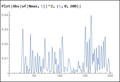
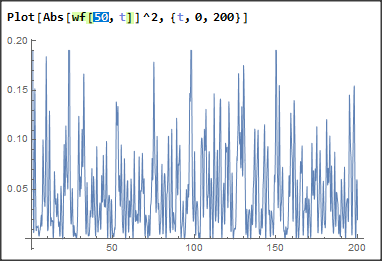
As your initial condition is a delta function, you have a lot of different momenta, what makes the wave function rather complicated. Here is a slice for x==50 and x==Nmax of Abs[psi]^2:

enter image description here

$\endgroup$
2
  • $\begingroup$ Add these two lines from above code ``` Pusol[t_] = (Re[usol[t]]^2 + Im[usol[t]]^2); ListDensityPlot[Table[Pusol[t][[i]], {t, tini, tmax}, {i, 1, Nmax}], PlotTheme -> "Scientific", FrameLabel -> {"n", "t"}, PlotLabel -> "[Sigma] =", PlotLegends -> Automatic] ``` this is the probability in time in x basis for a time independent Hamiltonian. I would like compare the same picture for time dependent Hamiltonian when the random numbers change at any time or failing that in a [Delta]t. If I understand your answer is like a Fourier Transform, right? $\endgroup$ Commented Apr 17, 2021 at 17:21
  • $\begingroup$ Sorry for the late answer. Abs[wf[t]]^2 and (Re[usol[t]]^2 + Im[usol[t]]^2) are the same thing, namely the position probability density. No, may answer is not a Fourier Transform, it is position, not momenta. If you change the Hamiltonian, usol changes, but the procedure above stays the same. $\endgroup$ Commented Apr 23, 2021 at 7:23

Your Answer

By clicking “Post Your Answer”, you agree to our terms of service and acknowledge you have read our privacy policy.

Not the answer you're looking for? Browse other questions tagged or ask your own question.