7
$\begingroup$

I'm quite new in Mathematica. I have a problem with obtaining the right solution for multi-layer 1D heat transfer problem. It seems that boundary condition not working. Could you advise something?

I would be obliged. Thank you in advance.

Clear["Global`*"]
Needs["NDSolve`FEM`"]

g = {0.25, 0.114, 0.04}; (*thickness *)
gw = Accumulate[g]
λ = {8, 1.8, 44};
ρ = {3100, 2100, 7800};
cp = {1050, 1100, 540};
dc = λ/(ρ*cp);
a = Piecewise[{{dc[[1]], x < gw[[1]]}, {dc[[2]], 
     gw[[1]] <= x < gw[[2]]}, {dc[[3]], x >= gw[[2]]}}, {x, 0, 
    gw[[3]]}];

σ = First[UnitConvert[Quantity["StefanBoltzmannConstant"]]];
Trob = 1700;
Tamb = 297;
h = 10;
ε = 0.85;

bc1 = DirichletCondition[T[t, x] == Trob, x == 0.];
bc2conv = NeumannValue[h*(Tamb - T[t, x]), x == gw[[3]]];
bc2rad = NeumannValue[ε*σ*(Tamb^4 - T[t, x]^4), 
   x == gw[[3]]];
ic1 = T[0, x] == Tamb;

pde = D[T[t, x], t] - a*D[T[t, x], x, x];

sol = NDSolveValue[{pde == bc2conv + bc2rad, bc1, ic1}, 
   T, {t, 0, 36000}, {x, 0., gw[[3]]}, MaxStepSize -> 50];

likzew


For the biggining thank you all for answer.

The 1D FEM model seems to me not very complicated, but I understand that neeed some clarificatrion. This is almost real situation. We have a three layers wall. Two part of them is ceramic materials (0.25m and 0.114m) , and last one is steel sheel (0.04 m). Using the Mathematica I trie to find solution which is sheel outside temperature after certain time. For t=0 s, temperature of whole wall is 297 degC. Boundary condition for x =0 is temperaturę Trob, boundary condition for x=0.404 contains convective and radiation therm. Simple and easy.

As wrote that is a almost real becouse I use some simplification for x=0 boundary condition. For that I should use heat floux rather than temperature bc. In real we have often more layers. I have also omit thermal conductivity temperaturę dependence. Becouse of thick ceramic layer with low thermal diffusivity I need solution for hours. That is why I calculate ht for 36000 s (10 hr) as example.

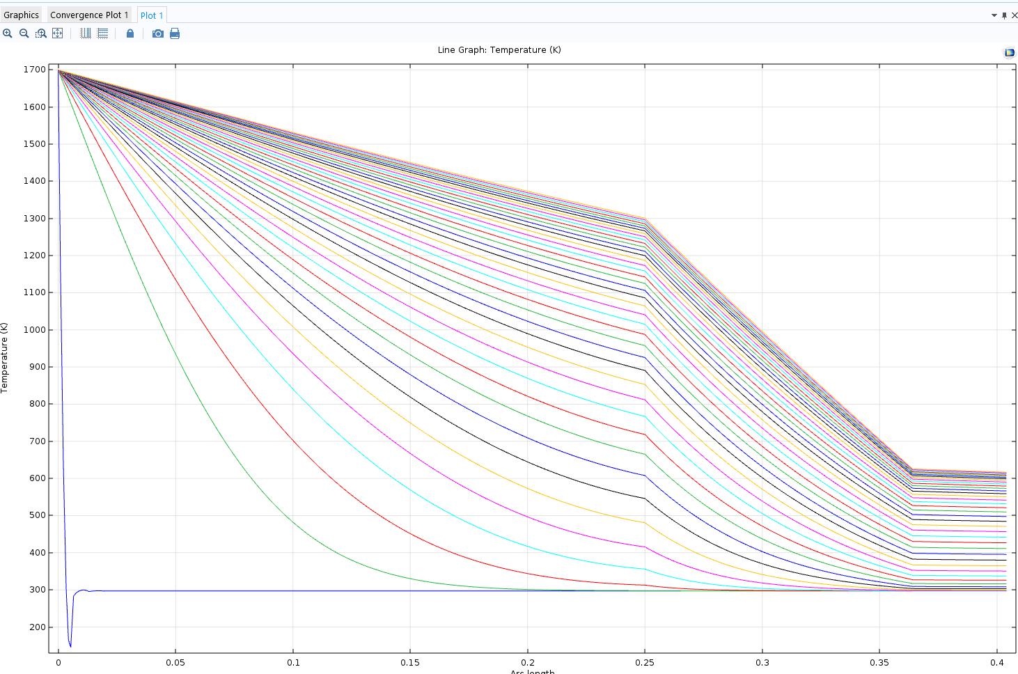
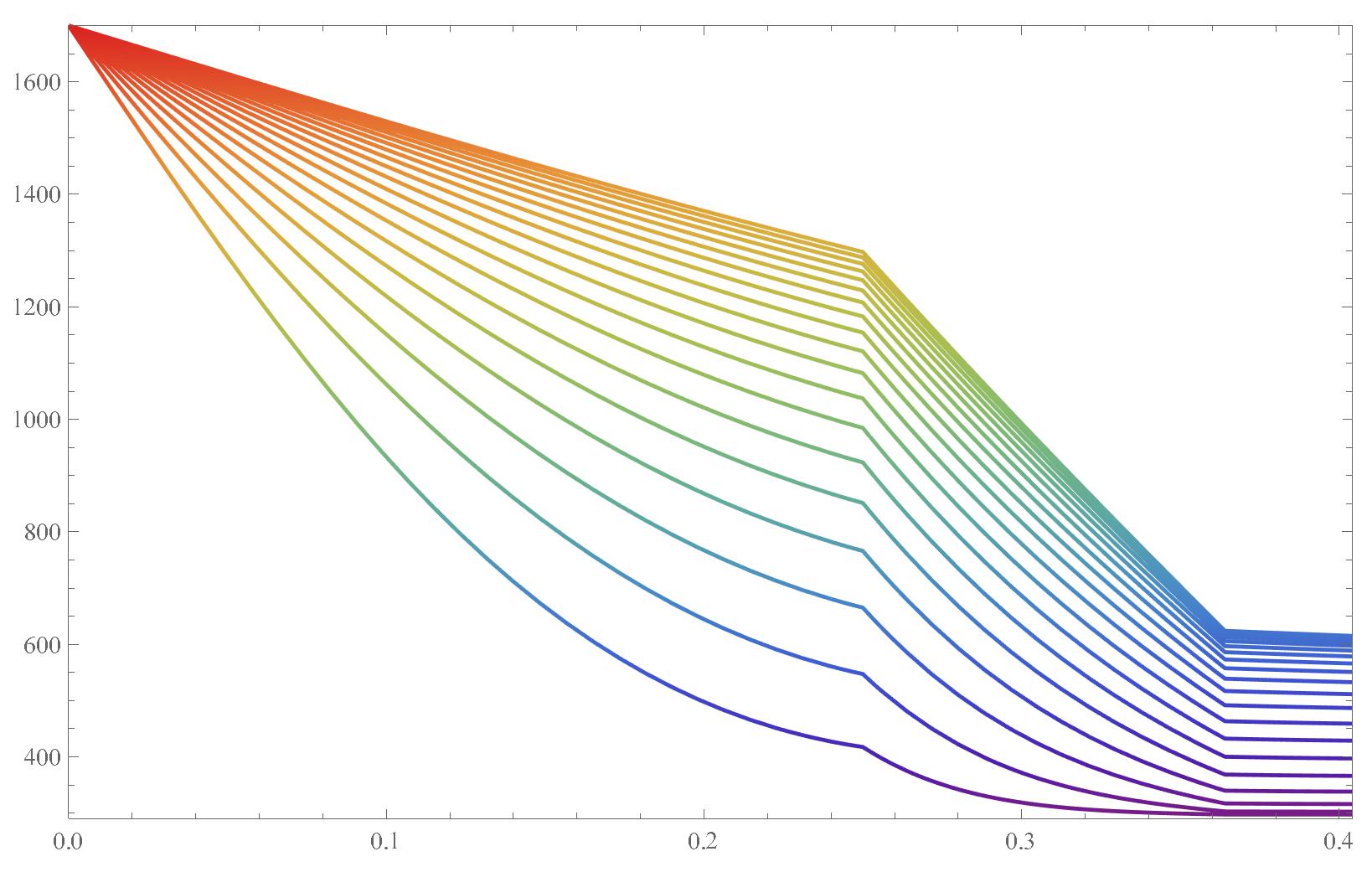
I enclose Comsol Multhiphisic 5.1 solution and my own solution obtained using Maple and method of lines which I delvelop a lot time ago. Both solution in range 0 - 36000 s (10 hr).

enter image description here

enter image description here

@xzczd

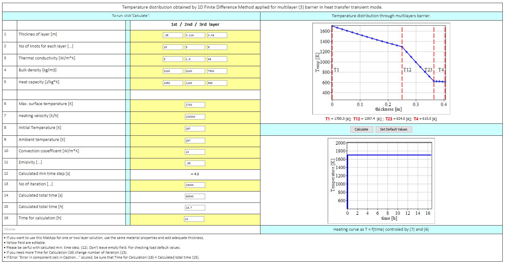
Here is a problem statement which I tried to solve using Mathematica. I am not sure if I was asked to do this.I am also not sure if this form is correct. But this is my definition of a problem.

enter image description here

=========================

Hmm...

I'm obviously doing something wrong in code.

Layer of steel, heated on one side (700degC, x = 0), on the other side (x = 10 cm) heat is picked up by convection (only). The result is obviously incorrect.

a = 44/(7840*560); (*steel*)
mesh = ToElementMesh[Line[{{0.}, {0.10}}], MaxCellMeasure -> 0.10/100];
pde = D[T[t, x], t] - a*D[T[t, x], x, x];
bc1 = DirichletCondition[T[t, x] == 700, x == 0.];
bc2 = NeumannValue[10*(297 - T[t, x]), x == 0.10];
ic1 = T[0, x] == 297;
sol = NDSolveValue[{pde == bc2, bc1, ic1}, T, {t, 0, 7200}, 
   x ∈ mesh, Method -> {"FiniteElement"}];
sol[7200, 0.10] (*=297K as T in t=0s*)

Results after 2h should be 691.2 K

Likzew

$\endgroup$
5
  • $\begingroup$ If I reduce the integration time to e.g. {t, 0, 100} I do obtain a solution, which can be plotted e.g. using Plot3D[sol[t, x], {t, 0, 100}, {x, 0, gw[[3]]}, PlotRange -> All] and looks reasonable. You may have to wait a looong time to get the full range you want. I also do get a weird Part error, but I am not sure where that comes from. What do you see? $\endgroup$
    – MarcoB
    Commented May 28, 2020 at 20:52
  • $\begingroup$ Hello, welcome to Mathematica.SE. Then, 1. You're imposing 3 boundary conditions, which is not correct. The bc2rad looks like the contribution of thermal radiation, if so, probably it should not be a NeumannValue, but an inhomogeneous term of heat conduction equation. You'd better show us the system in traditional math notation so we can help checking. 2. The continuity of heat flux is lost in your code, check these posts for more info: mathematica.stackexchange.com/q/131542/1871 mathematica.stackexchange.com/a/121739/1871 $\endgroup$
    – xzczd
    Commented May 29, 2020 at 1:30
  • 3
    $\begingroup$ There is a Heat Transfer tutorial that should be quite useful for your case. Have a look. Also, you can only have one boundary condition at a particular part of the boundary, you have two: bc2conv and bc2rad. In the heat transfer section of the PDEModels overview you can also find some heat transfer verification tests. $\endgroup$
    – user21
    Commented May 29, 2020 at 5:59
  • 1
    $\begingroup$ @likzew It could be better you post temperature on every border with time step 1000. Then we can compare solutions. $\endgroup$ Commented May 29, 2020 at 14:59
  • 1
    $\begingroup$ Version 13 has ToGradedMesh and ElementMeshRegionProduct. $\endgroup$
    – user21
    Commented Dec 16, 2021 at 8:03

3 Answers 3

6
$\begingroup$

I have not checked @Alex Trounev's answer, but this answer shows that there is good agreement between Mathematica and COMSOL Multiphysics.

Since you have a variety of thicknesses, I create a little routine so that I could mesh each region with the same number of elements (100 each).

Needs["NDSolve`FEM`"]
(* User Supplied Parameters *)
g = {0.25, 0.114, 0.04};(*thickness*)
gw = {0}~Join~Accumulate[g];
λ = {8, 1.8, 44};
ρ = {3100, 2100, 7800};
cp = {1050, 1100, 540};
(* Create a Multiregion Mesh *)
ClearAll[seg, appendCrdRight]
seg[thick_, nelm_, marker_] := Module[{crd, inc, marks},
  crd = Subdivide[0, thick, nelm];
  inc = Partition[Range[crd // Length], 2, 1];
  marks = ConstantArray[marker, inc // Length];
  <|"c" -> crd, "i" -> inc, "m" -> marks|>
  ]
appendCrdRight[a1_, a2_] := Module[{crd, inc, marks, len, lcrd},
  len = a1["c"] // Length;
  lcrd = a1["c"] // Last;
  inc = Join[a1["i"], a2["i"] + len - 1];
  crd = Join[a1["c"], Rest[a2["c"] + lcrd]];
  marks = Join[a1["m"], a2["m"]];
  <|"c" -> crd, "i" -> inc, "m" -> marks|>]
a = Fold[appendCrdRight, MapIndexed[seg[#1, 100, First[#2]] &, g]];
mesh = ToElementMesh["Coordinates" -> Partition[a["c"], 1], 
   "MeshElements" -> {LineElement[a["i"], a["m"]]}, 
   "BoundaryElements" -> {PointElement[{{1}, {a["c"] // Length}}, {1, 
       2}]}];
Show[mesh["Wireframe"["MeshElementStyle" -> {Red, Green, Blue}]], 
 PlotRange -> {-0.01, 0.01}]

Multiregion Mesh

Now, we can set up the PDE system and solve it on our newly created mesh.

σ = First[UnitConvert[Quantity["StefanBoltzmannConstant"]]];
Trob = 1700;
Tamb = 297;
h = 10;
ε = 0.85;
rhocp = Evaluate[
   Piecewise[{{ρ[[1]] cp[[1]], gw[[1]] <= x <= gw[[2]]},
     {ρ[[2]] cp[[2]], gw[[2]] <= x <= gw[[3]]},
     {ρ[[3]] cp[[3]], gw[[3]] <= x <= gw[[4]]}}]];
k = Evaluate[Piecewise[{{λ[[1]], gw[[1]] <= x <= gw[[2]]},
     {λ[[2]], gw[[2]] <= x <= gw[[3]]},
     {λ[[3]], gw[[3]] <= x <= gw[[4]]}}]];
bc1 = DirichletCondition[T[t, x] == Trob, x == 0];
bc2conv = NeumannValue[h*(Tamb - T[t, x]), x == Last@gw];
bc2rad = NeumannValue[ε*σ*(Tamb^4 - T[t, x]^4), 
   x == Last@gw];
ic1 = T[0, x] == Tamb;
op = Inactive[Div][{{-k}}.Inactive[Grad][T[t, x], {x}], {x}] + 
   rhocp*Derivative[1, 0][T][t, x];
pde = op == bc2conv + bc2rad;
sol = NDSolveValue[{pde, bc1, ic1}, 
   T, {t, 0, 36000}, {x} ∈ mesh, StartingStepSize -> 0.01];

The model I set up in COMSOL Multiphysics (v 5.5) shows similar results to those shown in the OP.
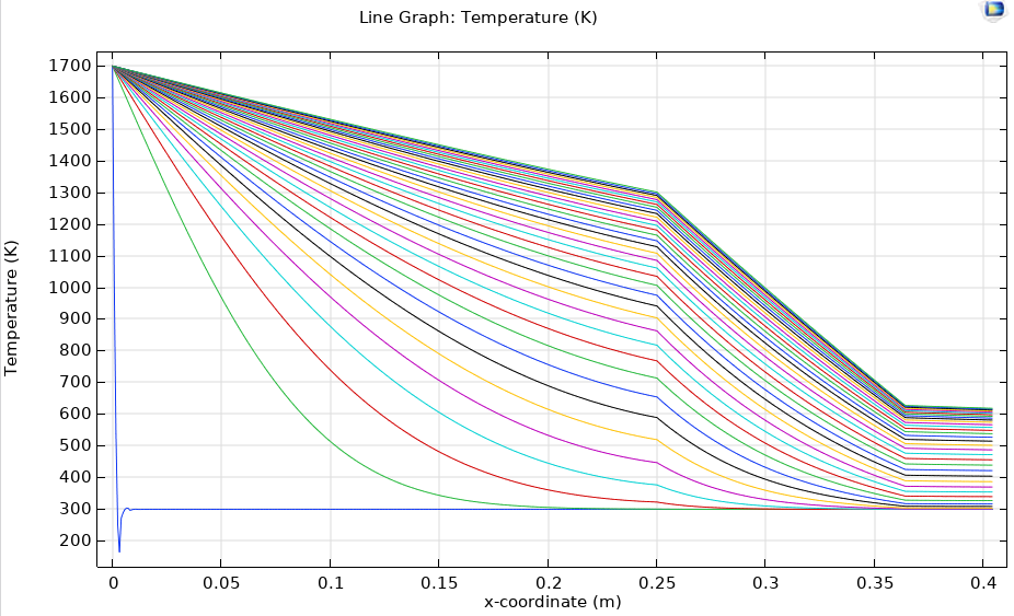
COMSOL Results

For comparison purposes, I extracted the temperature data at each phase boundary point in COMSOL.
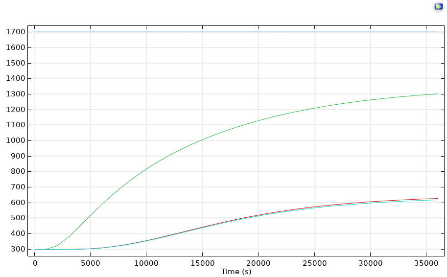
Temperature Data at Phase Boundaries

I exported these data to compare versus the Mathematica solution.

data = {{0, 1000, 2000, 3000, 4000, 5000, 6000, 7000, 8000, 9000, 
    10000, 11000, 12000, 13000, 14000, 15000, 16000, 17000, 18000, 
    19000, 20000, 21000, 22000, 23000, 24000, 25000, 26000, 27000, 
    28000, 29000, 30000, 31000, 32000, 33000, 34000, 35000, 
    36000}, {1700, 1700, 1700, 1700, 1700, 1700, 1700, 1700, 1700, 
    1700, 1700, 1700, 1700, 1700, 1700, 1700, 1700, 1700, 1700, 1700, 
    1700, 1700, 1700, 1700, 1700, 1700, 1700, 1700, 1700, 1700, 1700, 
    1700, 1700, 1700, 1700, 1700, 1700}, {297, 297.9169787`, 
    320.0562147`, 374.4552427`, 444.9013611`, 517.6131837`, 
    587.4876631`, 652.6604327`, 712.3644688`, 766.9603206`, 
    816.5391802`, 861.866491`, 902.8730203`, 940.4564489`, 
    974.5556695`, 1005.867455`, 1034.417079`, 1060.665637`, 
    1084.866141`, 1107.411419`, 1128.099762`, 1146.931167`, 
    1164.637928`, 1180.832645`, 1195.499525`, 1208.917884`, 
    1221.536363`, 1233.003818`, 1243.320249`, 1252.972747`, 
    1261.872597`, 1269.909554`, 1277.155111`, 1284.007597`, 
    1290.216067`, 1295.780522`, 1300.901468`}, {297, 297.0000101`, 
    297.0108185`, 297.2403045`, 298.3422144`, 301.3296677`, 
    306.8304462`, 315.0786727`, 326.0187665`, 339.0198185`, 
    353.9950315`, 370.1369655`, 387.5159699`, 405.1722292`, 
    423.1836315`, 440.8382141`, 458.14222`, 474.6735528`, 
    490.3439464`, 504.9171794`, 518.5145476`, 531.1360512`, 
    542.7808248`, 553.4493263`, 563.1415743`, 571.9455027`, 
    580.0023514`, 587.2015743`, 593.5431713`, 599.3724133`, 
    604.6264161`, 609.2270331`, 613.2390417`, 617.0233547`, 
    620.3526001`, 623.2267777`, 625.8287217`}, {297, 297.0000065`, 
    297.0084849`, 297.2058139`, 298.1991325`, 300.9831864`, 
    306.2034638`, 314.1201414`, 324.7019404`, 337.3400768`, 
    351.9481631`, 367.722907`, 384.7337123`, 402.0228897`, 
    419.6676093`, 436.9560503`, 453.8952359`, 470.0643493`, 
    485.3780489`, 499.6031165`, 512.8593059`, 525.1466173`, 
    536.4765686`, 546.8430665`, 556.2458626`, 564.7760878`, 
    572.5801167`, 579.5433842`, 585.6658902`, 591.2927421`, 
    596.3610853`, 600.7928104`, 604.6517643`, 608.293677`, 
    611.4944415`, 614.2540579`, 616.7511966`}};
Show[Plot[Evaluate[sol[t, #] & /@ gw], {t, 0, 36000}], 
 ListPlot[data[[2 ;; -1]], DataRange -> {0, 36000}]]
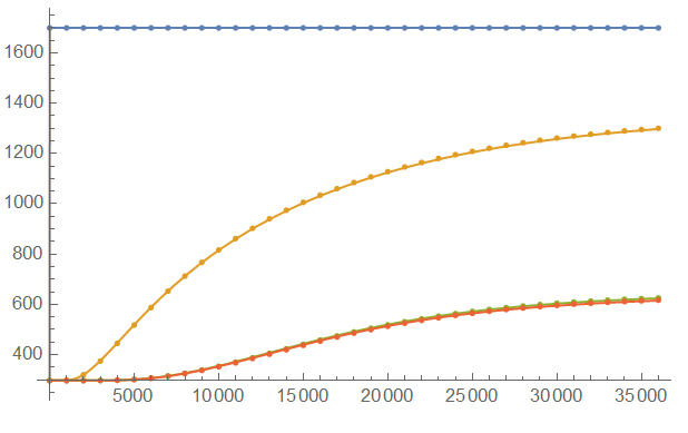
COMSOL Mathematica Comparison

As you can see, there is very little difference between COMSOL (dots) and Mathematica (solid lines).

Update to Include the Basic Form

@AlexTrounev requested a comparison of the basic form to COMSOL as defined by:

$$\rho {{\hat C}_p}\frac{{\partial T}}{{\partial t}} - \lambda \frac{{{\partial ^2}T}}{{\partial {x^2}}} = 0$$

To use the FEM method, I recommend to cast your equations into coefficient form as shown FEM Tutorial.

$$\frac{{{\partial ^2}}}{{\partial {t^2}}}u + d\frac{\partial }{{\partial t}}u + \nabla \cdot\left( { - c\nabla u - \alpha u + \gamma } \right) + \beta \cdot\nabla u + au - f = 0$$

I find it easier to make comparisons of commercial solver (such as COMSOL) results to Mathematica results.

As shown with the following workflow, the Alex's basic form also matches COMSOL quite closely. I also included a case where I tried to thermal diffusivity in coefficient form and it fails to match COMSOL. Finally, it may be interesting to note that COMSOL's Laplace Equation Interface does not contain a Laplacian, rather:

$$\nabla \cdot \left( { - \nabla u} \right) = 0$$

(* User Supplied Parameters *)
g = {0.25, 0.114, 0.04};(*thickness*)
gw = {0}~Join~Accumulate[g];
λ = {8, 1.8, 44};
ρ = {3100, 2100, 7800};
cp = {1050, 1100, 540};
σ = First[UnitConvert[Quantity["StefanBoltzmannConstant"]]];
Trob = 1700;
Tamb = 297;
h = 10;
ε = 0.85;
bmesh = ToBoundaryMesh["Coordinates" -> Partition[gw, 1], 
  "BoundaryElements" -> {PointElement[{{1}, {2}, {3}, {4}}]}]; nrEle \
= 100; pt = Partition[gw, 2, 1]; mesh = 
 ToElementMesh[bmesh, 
  "RegionMarker" -> 
   Transpose[{Partition[(Mean /@ pt), 1], {1, 2, 3}, 
     Abs[Subtract @@@ pt]/nrEle}]]
Show[mesh["Wireframe"["MeshElementStyle" -> {Red, Green, Blue}]], 
 PlotRange -> {-0.01, 0.01}]
rhocp = Evaluate[
   Piecewise[{{ρ[[1]] cp[[1]], gw[[1]] <= x <= gw[[2]]},
     {ρ[[2]] cp[[2]], gw[[2]] <= x <= gw[[3]]},
     {ρ[[3]] cp[[3]], gw[[3]] <= x <= gw[[4]]}}]];
k = Evaluate[Piecewise[{{λ[[1]], gw[[1]] <= x <= gw[[2]]},
     {λ[[2]], gw[[2]] <= x <= gw[[3]]},
     {λ[[3]], gw[[3]] <= x <= gw[[4]]}}]];
bc1 = DirichletCondition[T[t, x] == Trob, x == 0];
bc2conv = NeumannValue[h*(Tamb - T[t, x]), x == Last@gw];
bc2rad = NeumannValue[ε*σ*(Tamb^4 - T[t, x]^4), 
   x == Last@gw];
ic1 = T[0, x] == Tamb;
(* Coefficient Form *)
op = Inactive[Div][{{-k}}.Inactive[Grad][T[t, x], {x}], {x}] + 
   rhocp*Derivative[1, 0][T][t, x];
pde = op == bc2conv + bc2rad;
Tcoef = NDSolveValue[{pde, bc1, ic1}, 
   T, {t, 0, 36000}, {x} ∈ mesh, StartingStepSize -> 0.01];
(* Alex's "Basic Form" *)
op = rhocp*D[T[t, x], t] - k D[T[t, x], x, x];
pde = op == bc2conv + bc2rad;
Tbasic = NDSolveValue[{pde, bc1, ic1}, 
   T, {t, 0, 36000}, {x} ∈ mesh, StartingStepSize -> 0.01];
(* Coefficient form with thermal diffusivity *)
bc2conv = NeumannValue[h*(Tamb - T[t, x])/rhocp, x == Last@gw];
bc2rad = NeumannValue[ε*σ*(Tamb^4 - T[t, x]^4)/
     rhocp, x == Last@gw];
op = Inactive[Div][{{-k/rhocp}}.Inactive[Grad][T[t, x], {x}], {x}] + 
   Derivative[1, 0][T][t, x];
pde = op == bc2conv + bc2rad;
Talphainside = 
  NDSolveValue[{pde, bc1, ic1}, T, {t, 0, 36000}, {x} ∈ mesh,
    StartingStepSize -> 0.01];
(* Plot Alex's "Basic Form" *)
Show[Plot[Evaluate[Tbasic[t, #] & /@ gw], {t, 0, 36000}], 
 ListPlot[data[[2 ;; -1]], DataRange -> {0, 36000}]]
(* Comparison of Methods *)
Show[Plot[Evaluate[Tcoef[t, #] & /@ gw], {t, 0, 36000}, 
  PlotStyle -> ConstantArray[{Opacity[0.2], Thickness[0.015]}, 4]], 
 Plot[Evaluate[Talphainside[t, #] & /@ gw], {t, 0, 36000}, 
  PlotStyle -> Dashed], 
 Plot[Evaluate[Tbasic[t, #] & /@ gw], {t, 0, 36000}, 
  PlotStyle -> DotDashed]]
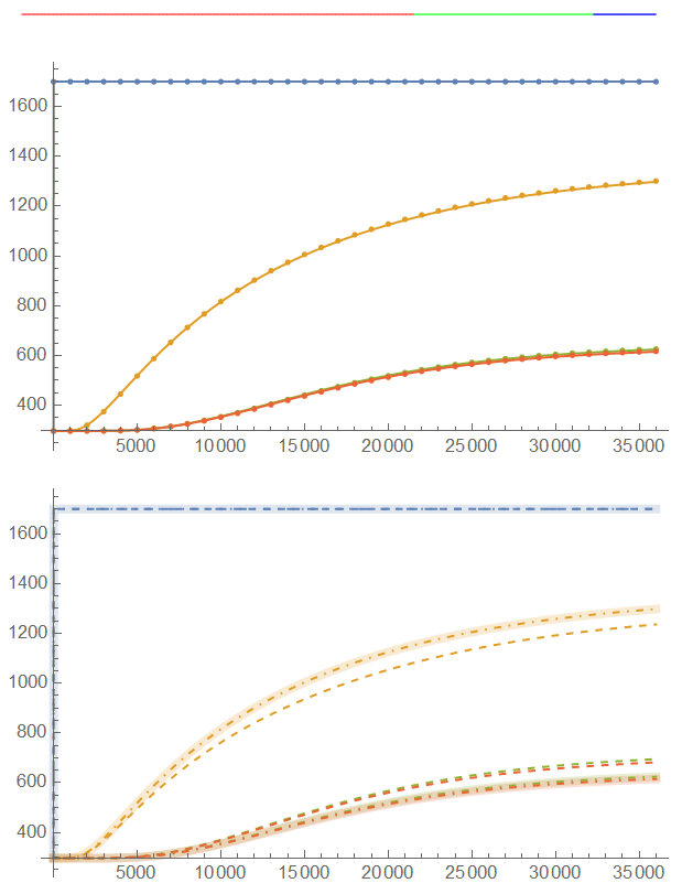
Basic Form

$\endgroup$
12
  • 1
    $\begingroup$ Excelent. Working very well. Thank you very much. $\endgroup$
    – likzew
    Commented Jun 1, 2020 at 5:06
  • $\begingroup$ Here is a shorter way to generate the mesh: bmesh = ToBoundaryMesh["Coordinates" -> Partition[gw, 1], "BoundaryElements" -> {PointElement[{{1}, {2}, {3}, {4}}]}]; nrEle = 10; pt = Partition[gw, 2, 1]; mesh = ToElementMesh[bmesh, "RegionMarker" -> Transpose[{Partition[(Mean /@ pt), 1], {1, 2, 3}, Abs[Subtract @@@ pt]/nrEle}]]; $\endgroup$
    – user21
    Commented Jun 1, 2020 at 7:18
  • $\begingroup$ @user21 Thanks. I was thrashing around trying to adapt a 2d bmesh to mesh approach to 1d, but it was getting late so I brute forced it. $\endgroup$
    – Tim Laska
    Commented Jun 1, 2020 at 13:08
  • $\begingroup$ @TimLaska Ok (+1)! You solve it in a basic form. But now check that in a question likzew asked about solution in a form of heat equation with a=frac{\lambda}{\rho c_p}$. And we know that it should be difference between two solutions. But we don't know what solution is right. Could you explain this? – Alex Trounev just now $\endgroup$ Commented Jun 2, 2020 at 11:14
  • 1
    $\begingroup$ @AlexTrounev Generally, to get the best correspondence between COMSOL and Mathematica, I put the expressions into coefficient form. For heat transfer in solids, COMSOL essentially solves $\rho {{\hat C}_p}\frac{{\partial T}}{{\partial t}} + \nabla \cdot {\mathbf{q}} = 0$, where $\mathbf{q}$ is the heat flux. That equation should be correct. In terms of temperature using Fourier's Law, it becomes $\rho {{\hat C}_p}\frac{{\partial T}}{{\partial t}} + \nabla \cdot \left( { - {\mathbf{k}}\nabla T} \right) = 0$. I don't think we can factor out conductivity when it is a function of $x$. $\endgroup$
    – Tim Laska
    Commented Jun 2, 2020 at 13:02
6
$\begingroup$

With a small modification of code we have

Needs["NDSolve`FEM`"]

g = {0.250, 0.114, 0.040};(*thickness*)gw = Total[g];
λ = {8, 1.8, 44};
ρ = {3100, 2100, 7800};
cp = {1050, 1100, 540};
dc = Table[λ[[i]]/(ρ[[i]]*cp[[i]])/10^-5, {i, 
    Length[cp]}];
a[x_] := Piecewise[{{dc[[1]], 0 <= x < g[[1]]}, {dc[[2]], 
    g[[1]] <= x < g[[2]] + g[[1]]}, {dc[[3]], True}}]

σ = 
  QuantityMagnitude[
    UnitConvert[Quantity["StefanBoltzmannConstant"]]] // N;
Trob = 1700.;
Tamb = 297;
h = 10;
ε = 0.85;

bc1 = DirichletCondition[
   T[t, x] == Exp[-1000 t] + Trob/Tamb (1 - Exp[-1000  t]), x == 0.];
bc2 = 10^5/(ρ[[3]] cp[[3]]) NeumannValue[
    h*(1 - T[t, x]) + ε*σ*Tamb^3 (1 - T[t, x]^4),
     x == gw];
bc2rad = NeumannValue[ε*σ*Tamb^3 (1 - T[t, x]^4),
    x == gw];
ic1 = T[0, x] == 1;

pde = D[T[t, x], t] - a[x]*D[T[t, x], x, x];
mesh = ToElementMesh[Line[{{0.}, {gw}}], MaxCellMeasure -> gw/404, 
  PrecisionGoal -> 5, AccuracyGoal -> 5]
sol = NDSolveValue[{pde == bc2, bc1, ic1}, T, {t, 0, .36}, 
  x ∈ mesh, Method -> {"FiniteElement"}]

(*Visualization *)

{Plot[a[x]/10^5, {x, 0, gw}, PlotRange -> All, Frame -> True, 
  AxesOrigin -> {0, 0}, Filling -> Axis], 
 Plot3D[Tamb sol[10^-5 t, x], {t, 0, 36000}, {x, 0., gw}, 
  AxesLabel -> Automatic, ColorFunction -> "Rainbow", Mesh -> None], 
 Plot[Table[Tamb sol[10^-5 t, x], {t, 2000, 36000, 2000}], {x, 0., 
   gw}, ColorFunction -> "Rainbow"]}

Figure 1

$\endgroup$
8
  • $\begingroup$ I think OP's question still needs clarification, see my comment above for more info. $\endgroup$
    – xzczd
    Commented May 29, 2020 at 1:36
  • 1
    $\begingroup$ @xzczd See update to my answer. $\endgroup$ Commented May 29, 2020 at 10:51
  • $\begingroup$ Thank you very much Alex. I tried to run your code, but I have obtained errors. I will look closer to why the problem occurs. But I counted however that I will able to solve this relatively easy FEM problem without any trick. As close to the definition of the problem as possible. $\endgroup$
    – likzew
    Commented May 29, 2020 at 18:42
  • $\begingroup$ @likzew Which version are you in? Nonlinear FEM is not supported before v12. $\endgroup$
    – xzczd
    Commented May 30, 2020 at 1:12
  • 2
    $\begingroup$ @likzew May be it means that Comsol solves equation in a basic form $\rho c_p \frac {\partial T}{\partial t}=\lambda \nabla^2 T$? $\endgroup$ Commented May 30, 2020 at 16:21
3
$\begingroup$

Once again, thank you to everyone who decided to help me in this calculation. As I wrote I have Mathematica since February 2020. I'm learning, but sometimes it's better to ask professionals.

Below is a solution that is based on MMA tutorials. Especially:

https://reference.wolfram.com/language/PDEModels/tutorial/HeatTransfer/HeatTransfer.html https://reference.wolfram.com/language/PDEModels/tutorial/HeatTransfer/ModelCollection/ShrinkFitting.html

I also used the elegant way of creating a 1D mesh given by @user21.

It should work.

Clear["Global`*"]
Needs["NDSolve`FEM`"]

HeatTransferModel[T_, X_List, k_, ρ_, Cp_, Velocity_, Source_] :=
  Module[{V, Q, a = k}, 
  V = If[Velocity === "NoFlow", 
    0, ρ*Cp*Velocity.Inactive[Grad][T, X]];
  Q = If[Source === "NoSource", 0, Source];
  If[FreeQ[a, _?VectorQ], a = a*IdentityMatrix[Length[X]]];
  If[VectorQ[a], a = DiagonalMatrix[a]];
  (*Note the-sign in the operator*)
  a = PiecewiseExpand[Piecewise[{{-a, True}}]];
  Inactive[Div][a.Inactive[Grad][T, X], X] + V - Q]
TimeHeatTransferModel[T_, TimeVar_, X_List, k_, ρ_, Cp_, 
  Velocity_, Source_] := ρ*Cp*D[T, {TimeVar, 1}] + 
  HeatTransferModel[T, X, k, ρ, Cp, Velocity, Source]

g = {0.25, 0.114, 0.04};
gw = {0}~Join~Accumulate[g];
bmesh = ToBoundaryMesh["Coordinates" -> Partition[gw, 1], 
  "BoundaryElements" -> {PointElement[{{1}, {2}, {3}, {4}}]}]; nrEle \
= 10; pt = Partition[gw, 2, 1]; mesh = 
 ToElementMesh[bmesh, 
  "RegionMarker" -> 
   Transpose[{Partition[(Mean /@ pt), 1], {1, 2, 3}, 
     Abs[Subtract @@@ pt]/nrEle}]];

ρ1 = 3100;
Cp1 = 1050;
k1 = 8;
ρ2 = 2100;
Cp2 = 1100;
k2 = 1.8;
ρ3 = 7800;
Cp3 = 540;
k3 = 44;

parameters = {ρ -> 
    Piecewise[{{ρ1, ElementMarker == 1}, {ρ2, 
       ElementMarker == 2}, {ρ3, ElementMarker == 3}}], 
   Cp -> Piecewise[{{Cp1, ElementMarker == 1}, {Cp2, 
       ElementMarker == 2}, {Cp3, ElementMarker == 3}}], 
   k -> Piecewise[{{k1, ElementMarker == 1}, {k2, 
       ElementMarker == 2}, {k3, ElementMarker == 3}}]};

σ = First[UnitConvert[Quantity["StefanBoltzmannConstant"]]];
Tamb = 297;
h = 10;
Trob = 1700;

bc2conv = NeumannValue[h*(Tamb - T[t, x]), x == 0.404];
bc2rad = NeumannValue[0.85*σ*(297^4 - T[t, x]^4), x == 0.404];
ic1 = {T[0, x] == Tamb};
bc1 = DirichletCondition[T[t, x] == Trob, x == 0];


pde = {TimeHeatTransferModel[T[t, x], t, {x}, k, ρ, Cp, "NoFlow",
       "NoSource"] == bc2conv + bc2rad, bc1, ic1} /. parameters;

sol = NDSolveValue[pde, T, {t, 0, 36000}, x ∈ mesh]

sol[36000, 0.404]

Plot[Table[sol[t, x], {t, 3600, 36000, 1800}], {x, 0, 0.404}, 
 PlotRange -> {{0, 0.404}, {290, 1700}}, PlotTheme -> "Scientific", 
 ColorFunction -> "Rainbow"]

Plot: {t,3600,36000,1800}

Likzew

$\endgroup$
1
  • $\begingroup$ So you use basic form of the heat equation while in your question you try to solve it in a form with a. It will be good if you change your question also to underlay this difference. $\endgroup$ Commented Jun 2, 2020 at 10:54

Your Answer

By clicking “Post Your Answer”, you agree to our terms of service and acknowledge you have read our privacy policy.

Not the answer you're looking for? Browse other questions tagged or ask your own question.