6
$\begingroup$

I have an interpolated function that looks like this:

$\hskip1.2in$enter image description here
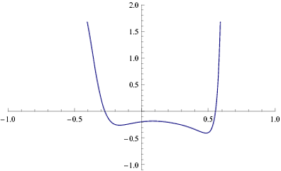
and, based on extreme and critical points, I want to use a polynomial to approximate the function. The points in question are:

pts = {{-0.405234, 1.67277}, {-0.163136, -0.261272}, {0.0847028, -0.183542},
    {0.483178, -0.408663}, {0.590177, 1.67277}};

$\hskip1.2in$enter image description here
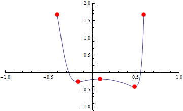
I know I could use Fit to get a polynomial with the desired order, but not every polynomial is acceptable.

In order to preserve the qualitative nature of the curve, the polynomial must be at least of order $n=4$, and a requirement is that the polynomial respects the minima of the original curve. Based on that, I did the following:

Let $P_4(x) = a_0 + a_1 x + a_2 x^2 + a_3 x^3 + a_4 x^4$. Then I constructed the function (sorry for the lousy programming)

p4[ls_] := Function[x, Module[{a, c4}, 
  a = Flatten@({a0, a1, a2, a3} /. 
  Solve[Flatten@{(a0 + a1 #1 + a2 #1^2 + a3 #1^3 + a4 #1^4 - #2 == 0) & @@@ #, 
    (a1 + 2 a2 #1 + 3 a3 #1^2 + 4 a4 #1^3 == 0) & @@@ #} &@ls[[{2, 4}]], 
    {a0, a1, a2, a3}]);
  c4 = a4 /. 
  (FindMinimum[
    Abs[a[[1]] + a[[2]] #1 + a[[3]] #1^2 + a[[4]] #1^3 + a4 #1^4 - #2] & @@ ls[[1]] +
    Abs[a[[1]] + a[[2]] #1 + a[[3]] #1^2 + a[[4]] #1^3 + a4 #1^4 - #2] & @@ ls[[3]] +
    Abs[a[[1]] + a[[2]] #1 + a[[3]] #1^2 + a[[4]] #1^3 + a4 #1^4 - #2] & @@ ls[[5]],
    {a4, 0}])[[2]];
  (a[[1]] + a[[2]] x + a[[3]] x^2 + a[[4]] x^3 + a4 x^4) /. {a4 -> c4}
  ]];

This function basically finds the coefficients $a_0, ...,a_3$ of the polynomial by imposing it to pass trough the two minima and ensuring that they are indeed minimia (fortunately I didn't had to impose $a_4 > 0$), and determines $a_4$ as the constant that minimizes the function

$$|P_4(x_1) - y_1| + |P_4(x_3) - y_3| + |P_4(x_5) - y_5|$$

The result is good but not that good:

$\hskip1.2in$enter image description here
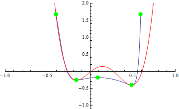
So, I try with $P_6(x) = a_0 + a_1 x + a_2 x^2 + a_3 x^3 + a_4 x^4 + a_5 x^5 + a_6 x^6$ (againg, sorry for the ugly programing):

p6[ls_] := Function[x, Module[{a, c6}, 
  a = Flatten@({a0, a1, a2, a3, a4, a5} /.
  Solve[Flatten@{(a0 + a1 #1 + a2 #1^2 + a3 #1^3 + a4 #1^4 
    + a5 #1^5 + a6 #1^6 - #2 == 0) & @@@ #,
    (a1 + 2 a2 #1 + 3 a3 #1^2 + 4 a4 #1^3 + 5 a5 #1^4 + 6 a6 #1^5 == 0) & @@@ #}
    &@ ls[[2 ;; 4]], {a0, a1, a2, a3, a4, a5}]);
  c6 = a6 /. (Quiet@FindMinimum[
     Abs[a[[1]] + a[[2]] #1 + a[[3]] #1^2 + a[[4]] #1^3 + a[[5]] #1^4 + 
     a[[6]] #1^5 + a6 #1^6 - #2] & @@ls[[1]] + 
     Abs[a[[1]] + a[[2]] #1 + a[[3]] #1^2 + a[[4]] #1^3 + a[[5]] #1^4 + 
     a[[6]] #1^5 + a6 #1^6 - #2] & @@ls[[3]] + 
     Abs[a[[1]] + a[[2]] #1 + a[[3]] #1^2 + a[[4]] #1^3 + a[[5]] #1^4 + 
     a[[6]] #1^5 + a6 #1^6 - #2] & @@ls[[5]], {a6, 0}])[[2]];
  (a[[1]] + a[[2]] x + a[[3]] x^2 + a[[4]] x^3 + a[[5]] x^4 + a[[6]] x^5 + a6 x^6) /.
     {a6 -> c6}
]];

Again I force the minima, but I add a third condition on the coeficients, that there must be a minima in $x_3$. This works like a charm for pts:

$\hskip1.2in$enter image description here
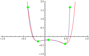
I should be very happy but, if I change the definition for pts

pts = {{-0.419826, 1.67277}, {-0.292539, -0.296446}, {0.00452181, -0.162576}, 
  {0.6037, -0.534627}, {0.735329, 1.67277}}

I end up with

$\hskip1.2in$enter image description here
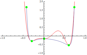
which is terrible (qualitatively speaking that is)!

The solution is (kinda?) obvious, I need to impose the constraint

$$2 a_2 + 6 a_3 x + 12 a_4 x^2 + 20 a_5 x^3 + 30 a_6 x^4 \le 0 \quad x \in (x_2 + \delta_1,x_4 - \delta_2) \tag{C}$$

(where $\delta_{1,2}$ can be fixed to ensure smoothness) but I have been unable to work with the interval. I've tried defining a function by pieces and apply it to $a_6$ in the constraint section of FindRoot, use HeavisidePi, etc, without success so, my quiestion is: how to include the constraint (C) in FindRoot?

For reference, here is a (coarse) table to generate the original interpolated function for the first and second case:

case1 = {{-0.405234, 1.67277}, {-0.305234, 0.264728}, {-0.205234, -0.2388},
   {-0.105234, -0.242507}, {-0.00523355, -0.197663}, {0.0947664, -0.183713},
   {0.194766,-0.203222}, {0.294766, -0.252936}, {0.394766, -0.334333},
   {0.494766, -0.404536}};

case2 = {{-0.419826, 1.67277}, {-0.319826, -0.275709}, {-0.219826, -0.248922},
   {-0.119826, -0.185553}, {-0.0198259, -0.163342}, {0.0801741, -0.169325},
   {0.180174, -0.197047}, {0.280174, -0.244685}, {0.380174, -0.313329},
   {0.480174, -0.41021}, {0.580174, -0.524263}, {0.680174, -0.190625}};

Thanks for the attention.

$\endgroup$
4
  • 2
    $\begingroup$ I am not able to see how that last solution is "terrible": it has done all you ask of it. Because your input (red) curve apparently enjoys few or no restrictions, you cannot expect a polynomial of any degree to fit that curve closely between the sampled points, except by pure luck. This seems like a losing game you're playing, unless you know something about the red curve that you're not sharing with us. BTW, if by "$x_2$ you mean the second point from the left, etc., then condition (C) is inconsistent with $x_2$ and $x_4$ being smooth local minima. $\endgroup$
    – whuber
    Commented Mar 19, 2013 at 0:07
  • $\begingroup$ @whuber It behaves "terribly" because is intorducing new local maxima and minima, and this is a problem because additional maxima and minima means spurious stationary solutions when working whit dynamical systems. The fourth order polynomial does a good job, but the original curves case1 and case2 are taken from actual data, and it's very important to see if I can improve the fit (n=6). You're right about the condition on (C) and I've modified it accordingly. $\endgroup$
    – Pragabhava
    Commented Mar 19, 2013 at 3:43
  • $\begingroup$ Polynomials are virtually guaranteed to do that: after all, a degree $d$ polynomial will typically have $d-1$ critical points. Your new condition (C) has two problems: a minor one is the typographical error (it should be degree $4$, not $5$) but the more serious is that it is ill-defined, because $\delta_1$ and $\delta_2$ are unspecified, and therefore the constraint is difficult (or impossible) to make operational. Why not consider using a different family of functions for your fits, such as splines? $\endgroup$
    – whuber
    Commented Mar 19, 2013 at 4:08
  • $\begingroup$ @whuber You are right. I meant to manually input the $\delta_{1,2}$; sorry for the confusion. $\endgroup$
    – Pragabhava
    Commented Mar 19, 2013 at 14:01

1 Answer 1

5
$\begingroup$

I share the objections made by whuber, but I like that you put quite a bit of effort into the question. Let me explain one detail of whubers comment with an example before giving you a possible solution

it has done all you ask of it

When using interpolation, exactly this is the point many people don't consider when they see interpolating functions which behave badly. All you ask is, that your functions matches the data-points, what happens in between is not stated. Especially higher order polynomial tend to contain ringing artifacts and therefore, the specified points match exactly, but the interpolation looks ugly nevertheless. Exactly this happened to you.

You can now try to specify more and more constraints ending up with even higher polynomials and you would be surprised how creative ideas your function will develop to do exactly the opposite of what you want in places you haven't specified.

One possible way out is to specify a global distance measure between your interpolating function and your polynomial you try to find. First let's interpolate your points

ip = Interpolation[
   case2 = {{-0.419826, 
      1.67277}, {-0.319826, -0.275709}, {-0.219826, -0.248922}, \
{-0.119826, -0.185553}, {-0.0198259, -0.163342}, {0.0801741, \
-0.169325}, {0.180174, -0.197047}, {0.280174, -0.244685}, {0.380174, \
-0.313329}, {0.480174, -0.41021}, {0.580174, -0.524263}, {0.680174, \
-0.190625}}, Method -> "Spline"];
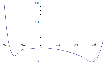
Plot[ip[x], {x, -.4, .7}, PlotRange -> All]

Mathematica graphics

To compare now this interpolating function with an yet unknown polynomial, we could integrate the (squared) difference over the region, but since a numerical integration with step control and all the fancy stuff is slower than adding up some numbers, we will calculate the difference only on some discrete places. For this, we sample ip with significantly more points than we initially had

{xs, ys} = Transpose@Table[{x, ip[x]}, {x, -.4, .7, 0.001}];

Let's say we have a polynomial depending on factors $a_i$, then we want to be able to compute the difference between polynomial and our sample points very fast. The squared difference is something along

$$\left(\left(a_1+\sum_{i=2}^n a_i\cdot x^{i-1}\right)-y\right)^2$$

for each point {x,y}. A list-parallel compiled function will serve us well

sqrdDiff = Compile[{{x, _Real, 0}, {y, _Real, 0}, {a, _Real, 1}},
  (a[[1]] + Sum[a[[i]]*x^(i - 1), {i, 2, Length[a]}] - y)^2
  , CompilationTarget -> "C", Parallelization -> True, 
  RuntimeAttributes -> {Listable}
];
targetFunc[parms : {_?NumericQ ..}] := Total@sqrdDiff[xs, ys, parms];

The targetFunc is only there to force that sqrDiff is only called with numerical $a_i$ and to calculate the sum of all difference in the points.

Now calculating a polynomial of degree 15 is a small step

n = 15;
With[{parms = Array[a, n]},
 sol = Last@NMinimize[
    targetFunc[parms], parms]
 ]

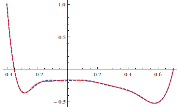
and using the values for a[i] in sol we can plot everything together

Plot[Evaluate[
  {Sum[a[i]*x^(i - 1), {i, n}] /. sol,
   ip[x]}], {x, -.4, .7}, 
 PlotStyle -> {Directive[Thick, Dashed], Directive[Red]},
 PlotRange -> All]

Mathematica graphics

$\endgroup$
6
  • $\begingroup$ +1 I love the "creative ideas" passage. To anticipate the next objection: don't try to extrapolate this fit! Another thought: once you get up to degree 15, why don't you just use a spline? It would have as many free parameters and likely be easier to fit. $\endgroup$
    – whuber
    Commented Mar 19, 2013 at 3:18
  • 1
    $\begingroup$ @whuberThanks. Here, I was using an ordinary polynomial just because the OP wants one. Honestly, I doubt that he really seeks one closed polynomial form, but we won't know until he explains what he wants to do with it. Maybe he gives some more details when he reads this. $\endgroup$
    – halirutan
    Commented Mar 19, 2013 at 3:28
  • $\begingroup$ @whuber and halirutan First of all, thanks for taking the time. Maybe it's just me, but I feel like I'm being dumbed out. There are very good reasons why I need a low order polynomial: one is for analytical work, (where splines or hidden InterpolatingFunction are wortless); other is that I'm traking some zeros using the original data, and is very expensive to find all the solutions, which are strongly related to the maxima and minima. I know that, qualitatively, a polynomial with the w shape will give the correct information of the system, as long as it is a good approximation. $\endgroup$
    – Pragabhava
    Commented Mar 19, 2013 at 4:14
  • $\begingroup$ Well, at a minimum you need to use an appropriate degree. If you want to fit five points and three derivatives exactly, you need at least a seventh degree polynomial--there's no way around that unless you get lucky. But "w shape" is sufficiently vague that in general you don't have much hope of fitting it well with a polynomial unless the degree is much higher, in which case it will exhibit spurious behaviors, as halirutan so ably describes here. $\endgroup$
    – whuber
    Commented Mar 19, 2013 at 4:18
  • $\begingroup$ @Pragabhava And I had hoped, that you have your reasons. Have you tried using my approach with n=5 and many sampling points? I get here a result that looks like i.sstatic.net/GlzSN.png Would that be sufficient? $\endgroup$
    – halirutan
    Commented Mar 19, 2013 at 11:40

Your Answer

By clicking “Post Your Answer”, you agree to our terms of service and acknowledge you have read our privacy policy.

Not the answer you're looking for? Browse other questions tagged or ask your own question.