Progress can be made by integrating over y only (with the correction that {…} be replaced by (…)).
Integrate[x DiracDelta[r x - y] Exp[1/g^2 (Cos[x2 - x] + Cos[x2] + Cos[y + x2])],
    {y, 0, 2 Pi}, Assumptions -> r > 0 && 0 < x < 2 Pi]
(* E^((Cos[x - x2] + Cos[x2] + Cos[r x + x2])/g^2) x HeavisideTheta[2 Pi - r x] *)
In contrast, if r < 0, the result is 0, as one would expect.
The remaining integrals take the form,
Integrate[E^((Cos[x - x2] + Cos[x2] + Cos[r x + x2])/g^2)
    x HeavisideTheta[2 Pi - r x], {x, 0, 2 Pi}, {x2, -Pi, Pi}]
Edit: which can be simplified further to
Integrate[E^((Cos[x - x2] + Cos[x2] + Cos[r x + x2])/g^2) x,
    {x, 0, 2 Pi Min[1, 1/r]}, {x2, -Pi, Pi}
Now, if g^2 is much greater than 1, then the remaining integrations can be performed with the exponential ignored.
Integrate[x, {x, 0, 2 Pi Min[1, 1/r]}, {x2, -Pi, Pi}, Assumptions -> r > 0]
(* (4 Pi^3 Min[1, 1/r]^2 *)
For g^2 not large, the remaining integrals must be performed numerically along the lines suggested by Alx in a comment above, but a 2D plot is slow.
f[r_?NumericQ, g_?NumericQ] := NIntegrate[E^((Cos[x - x2] + Cos[x2] + Cos[r x + x2])/g^2) x,
    {x, 0, 2 Pi Min[1, 1/r]}, {x2, -Pi, Pi},
    Method -> {Automatic, "SymbolicProcessing" -> False}]
A 1D plot for g == 1 is
Plot[f[r, 1], {r, 0, 4}, MaxRecursion -> 2, ImageSize -> Large,
    AxesLabel -> {r, None}, LabelStyle -> {15, Bold, Black}]
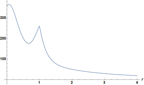
For a small value of g, the curve is somewhat different.
LogPlot[f[r, 1/10], {r, 0, 4}, MaxRecursion -> 3, ImageSize -> Large,
    AxesLabel -> {r, None}, LabelStyle -> {15, Bold, Black}, PlotRange -> All]
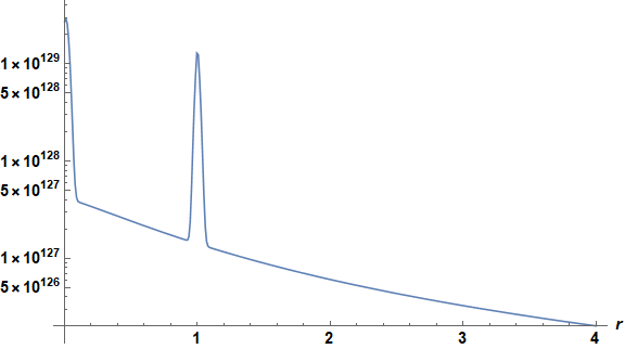
Peaks lie at r = 1 and very close to r = 0.
Addendum
The further simplification identified by Andreas (+1), equivalent to
f[r_?NumericQ, g_?NumericQ] := 2 Pi NIntegrate[BesselI[0, g^-2
    Sqrt[3 + 2 Cos[x] + 2 Cos[r x] + 2 Cos[(1 + r) x]]] x, {x, 0, 2 Pi Min[1, 1/r]},
    Method -> {Automatic, "SymbolicProcessing" -> False}]
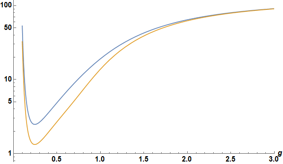
reproduces the plots above about an order of magnitude faster. For completeness, we provide a plot of the values at the two peak values as functions of g (rescaled by Exp[-2.94 g^-2] to keep the curves readable.
LogPlot[{f[.02, g] Exp[-2.94 g^-2], f[1, g] Exp[-2.94 g^-2]}, {g, 1/10, 3},
    ImageSize -> Large, AxesLabel -> {g, None}, LabelStyle -> {15, Bold, Black},
    PlotRange -> {{0, 3}, Automatic}]
The blue and orange curves correspond to r = 0.02 and r = 1, respectively.


f[r_?NumericQ, g_?NumericQ]:=NIntegrate[...]. $\endgroup$Plot3D[f[r,g],{r,...},{g,...}], you need to put in ranges forrandg. $\endgroup$