2
$\begingroup$

i have put up and question about the NDSolve and have got the solution of the ODE,and also got the figure of t1-t ,however when i use the solution of the t1-t to integrate ,the integral didn't converge and the figure of the p1 is continous but when i export the p1 result to the EXCEL,the figure is Discontinuous,so how to deal with it?

the related questions

NDSolve will try solving the system as differential-algebraic equations but it didn't get the solution

and i have Extract the equation of the original question and

codes are as this

equa00 = 0.` - \[Piecewise] {
  {2 x''[t] + 1/2 (4900.` + 259 x''[t] + 2 (4900.` + 500 x''[t])),
    x'[t] >= 0},
  {4900.` + 503 x''[t], x'[t] < 0},
  {0, \!\(\*
     TagBox["True",
      "PiecewiseDefault",
      AutoDelete->False,
      DeletionWarning->True]\)}
 } + 159715.5` (0.25` Cos[1.7951958020513104` t] - x[t]) - 
13130.602263408473` Cos[
  1.7951958020513104` t] (0.613591041570793` + 
   0.25` Cos[1.7951958020513104` t] - x[t]) + 
6519.` Abs[-0.4487989505128276` Sin[1.7951958020513104` t] - 
   x'[t]] (-0.4487989505128276` Sin[1.7951958020513104` t] - 
   x'[t]) + 16297.5` (\[Piecewise] {
    {0.56796693652872623432387422799011`31.754323054547157, 
     x'[t] >= 0},
    {0.49855266876742266072254490600473`31.69771104538948, 
     x'[t] < 0},
    {0, \!\(\*
       TagBox["True",
        "PiecewiseDefault",
        AutoDelete->False,
        DeletionWarning->True]\)}
   }) (0.613591041570793` + 0.25` Cos[1.7951958020513104` t] - 
   x[t]) (-0.8056819919256618` Cos[1.7951958020513104` t] - 
   x''[t]) == 10000 x''[t];


t1 = \[Piecewise] {
{2 x''[t] + 1/2 (4900 + 259 x''[t] + 2 (4900 + 500 x''[t])), 
 x'[t] >= 0},
{4900 + 503 x''[t], x'[t] < 0},
{0, \!\(\*
   TagBox["True",
    "PiecewiseDefault",
    AutoDelete->False,
    DeletionWarning->True]\)}
   };

t0 = 100;
s1 = NDSolve[{equa00, x[0] == 1, x'[0] == 1}, x, {t, 0, t0}, 
  SolveDelayed -> True]

p1 = (t1 /. s1)*(x[t] /. s1);
Plot[p1, {t, 0, t0}, PlotRange -> All]

period = 23.14;

paverage = NIntegrate[p1, {t, 40, 40 + period}]/period

i just want to integrate the p1,however it doesn't converge

NIntegrate::slwcon: Numerical integration converging too slowly; suspect one of the following: singularity, value of the integration is 0, highly oscillatory integrand, or WorkingPrecision too small. >>
NIntegrate::ncvb: NIntegrate failed to converge to prescribed accuracy after 9 recursive bisections in t near {t} = {43.7509}. NIntegrate obtained -7211.41 and 23.400613386693852` for the integral and error estimates. >>

the result is

{-311.643}
$\endgroup$
3
  • $\begingroup$ Welcome to Mathematica.SE, dcydhb! I suggest the following: 1) Take the tour and check the faqs. 2) When you see good questions and answers, vote them up by clicking the gray triangles, because the credibility of the system is based on the reputation gained by users sharing their knowledge. Also, please remember to accept the answer, if any, that solves your problem, by clicking the checkmark sign! 3) As you receive help, try to give it too, by answering questions in your area of expertise. $\endgroup$
    – Chris K
    Commented Nov 6, 2019 at 9:32
  • $\begingroup$ @Chris K,in fact when there are more than 2 answers and they all can solve my questions,i don't konw how to select and in fact i want to select them all. $\endgroup$
    – dcydhb
    Commented Nov 6, 2019 at 11:47
  • $\begingroup$ Yeah that can be hard to decide. In any case, there is no limit to the number of answers that you can upvote with the gray triangle. $\endgroup$
    – Chris K
    Commented Nov 6, 2019 at 12:37

2 Answers 2

5
$\begingroup$

Simply increasing the MaxRecursion gives an answer without the NIntegrate::ncvb message:

paverage = 
 NIntegrate[p1, {t, 40, 40 + period}, MaxRecursion -> 100]/period
(* {-311.506} *)

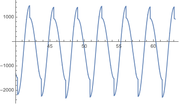
BTW, looking at your function over this range, it does not look like the period is 23.14.

Plot[p1, {t, 40, 40 + period}]

Mathematica graphics

EDIT: Extra method

@MichaelE2's answer is so nice it motivates me to improve mine a little. So here's an alternative, NIntegrate-free approach, that solves for the integral within the NDSolve:

s1 = NDSolve[{equa00, intp1'[t] == t1*x[t], x[0] == 1, x'[0] == 1,
  intp1[0] == 0}, {x, intp1}, {t, 0, t0}, SolveDelayed -> True]

(intp1[40 + period] - intp1[40])/period /. s1[[1]]
(* -311.513 *)

$\endgroup$
5
  • $\begingroup$ yes,the real period is not 23.14,it doesn't matter this question,and NIntegrate::slwcon: Numerical integration converging too slowly; suspect one of the following: singularity, value of the integration is 0, highly oscillatory integrand, or WorkingPrecision too small. >> still exist,it means the result is not accurate or it only means the Convergence is slow ? $\endgroup$
    – dcydhb
    Commented Nov 6, 2019 at 9:18
  • $\begingroup$ and if the real solution of p1 is continous,will the figure of p1 is continous means the solution of p1 is continus? why when i export p1 data to EXCEL and plot in EXCEL,the figure is discontinous? $\endgroup$
    – dcydhb
    Commented Nov 6, 2019 at 9:21
  • $\begingroup$ NIntegrate::slwcon is a warning, not an error. If you get an answer without NIntegrate::ncvb it should be good. Sorry, I have no idea about your plot in Excel. $\endgroup$
    – Chris K
    Commented Nov 6, 2019 at 9:30
  • $\begingroup$ you have solved my question and thanks a lot! $\endgroup$
    – dcydhb
    Commented Nov 6, 2019 at 10:19
  • $\begingroup$ @dcydhb I believe p1 is discontinuous when x'[t] == 0. Plot cannot figure that out on its own. Compare with Plot[p1, {t, 40, 44}, PlotRange -> All, Exclusions -> (x'[t] == 0 /. First@s1)]. $\endgroup$
    – Michael E2
    Commented Nov 6, 2019 at 12:50
5
$\begingroup$

An InterpolatingFunction has weak singularities at each point of the interpolating grid. They confound the default integration rules, which are a based on the assumption that the integrand is smooth. You can specify the singularities sometimes with Method -> "InterpolationPointsSubdivision", but it does not work here, maybe because of the complexity of p1. You can also list them explicitly in the iterator that specifies the domain of integration.

sing = Flatten[x["Grid"] /. s1]; (* the interpolation grid *)

With[{iter =  (* add the relevant singularities to the iterator *)
   Flatten@{t, 40, Select[sing, 40 < # < 40 + period &], 40 + period}},
 paverage = NIntegrate[p1, iter]/period
 ]
(*  {-311.513}  *)

Update

OK, currently this answer has more upvotes than @ChrisK's. While that answer does not explain why it works, Chris's approach does handle the integral more effectively than my way above. I can explain why.

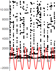
There are two sources of truncation error in the numerical integration. One comes from the weak singularities that mentioned above. Another, that I mentioned only in a comment, comes from discontinuities in p1 at the points where x'[t] == 0. Further investigation shows these are more significant than the weak singularities I mentioned (and there are 6000+ of them). The setting MaxRecursion -> 100 may seem overkill, but it allows NIntegrate to resolve (quickly, in fact) the error at the discontinuities. The error from the weak singularities does not matter that much because the interpolation grid is so fine that those errors are not that great.

Here's how to see what is going on in Chris's solution:

Needs["Integration`NIntegrateUtilities`"]

Show[
 NIntegrateSamplingPoints@
  NIntegrate[p1, {t, 40, 40 + period}, MaxRecursion -> 100],
 Plot[5000 x'[t] /. s1, {t, 40, 40 + period}, PlotStyle -> Red],
 PlotRange -> All]

enter image description here

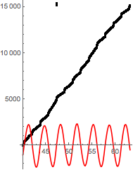
We can see that the sampling is concentrated along the lines where x'[t] == 0. Every now and then the intervals between these roots are subdivided and resampled. This happens when the error from the discontinuities becomes less than the error from the weak singularities (this is the global adaptive strategy). If we do the same analysis on my code, we see that there is very little recursive subdivision with about 50% more sampling points -- and it takes ten times as long. That time can be cut in half with Method -> {"GlobalAdaptive", "SymbolicProcessing" -> 0}.

Show[
 With[{iter = 
    Flatten@{t, 40, Select[sing, 40 < # < 40 + period &], 40 + period}},
  NIntegrateSamplingPoints@NIntegrate[p1, iter]
  ],
 Plot[5000 x'[t] /. s1, {t, 40, 40 + period}, PlotStyle -> Red],
 PlotRange -> All]

enter image description here

$\endgroup$

Your Answer

By clicking “Post Your Answer”, you agree to our terms of service and acknowledge you have read our privacy policy.

Not the answer you're looking for? Browse other questions tagged or ask your own question.