To solve the problem, we can apply FEM using explicit Euler in time. So that there were no messages, we organized a weak leak across the border.
Needs["NDSolve`FEM`"]; t1 = 2; \[CapitalDelta]\[Phi] =
 40/180 Pi ; r1 = 0.161; r2 = 0.201; \[Lambda] = 1/2;
f[x_] := Piecewise[{{50 , 0 <= x <= \[CapitalDelta]\[Phi]}, {0,
    True}}]; mesh = ImplicitRegion[r1^2 <= x^2 + y^2 <= r2^2, {x, y}];
t0 = 1/20; n = 40;
U[0][x_, y_] := 100;
Do[U[t] =
   NDSolveValue[(u[x, y] - U[t - t0][x, y])/
       t0 - \[Lambda] Laplacian[u[x, y], {x, y}] + (x D[u[x, y], y] -
        y D[u[x, y], x]) - f[ArcTan[x, y]] + 0.025 (u[x, y] - 20) ==
     NeumannValue[10^-9 u[x, y], True], u, {x, y} \[Element] mesh,
    Method -> {"FiniteElement", InterpolationOrder -> {u -> 2},
      "MeshOptions" -> {"MaxCellMeasure" -> 0.001,
        "MeshOrder" -> 2}}];, {t, t0, n t0, t0}]
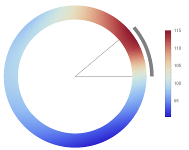
Table[DensityPlot[Evaluate[U[t][x, y]], {x, y} \[Element] mesh,
  PlotLegends -> Automatic, PlotLabel -> Row[{"t = ", t*1.}],
  ColorFunction -> ColorData["ThermometerColors"], PlotPoints -> 100,
  Frame -> False, ColorFunctionScaling -> True], {t, 10 t0, n*t0,10 t0}]
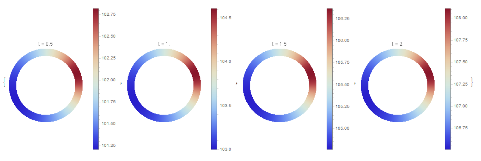 For comparison, we used the 1D model, given the absence of gradients along
 r. We see that the data is consistent with FEM.
With[{r = (r1 + r2)/2},
 U1 = NDSolveValue[{Derivative[1, 0][u][t, \[CurlyPhi]] +
      Derivative[0, 1][u][
       t, \[CurlyPhi]] == \[Lambda] D[
         u[t, \[CurlyPhi]], {\[CurlyPhi], 2}]/r^2 + f[\[CurlyPhi]] -
      0.025 (u[t, \[CurlyPhi]] - 20), u[0, \[CurlyPhi]] == 100,
    u[t, 0] == u[t, 2 Pi]}, u, {\[CurlyPhi], 0, 2 Pi}, {t, 0, t1},
   Method -> {"MethodOfLines",
     "SpatialDiscretization" -> {"TensorProductGrid",
       "MinPoints" -> 200, "MaxPoints" -> 200,
       "DifferenceOrder" -> 4}}]]

Table[DensityPlot[
  Evaluate[U1[t, ArcTan[x, y]]], {x, y} \[Element] mesh,
  PlotLegends -> Automatic, PlotLabel -> Row[{"t = ", t*1.}],
  ColorFunction -> ColorData["ThermometerColors"], PlotPoints -> 100,
  Frame -> False, ColorFunctionScaling -> True], {t, 10 t0, n*t0,
  10 t0}]
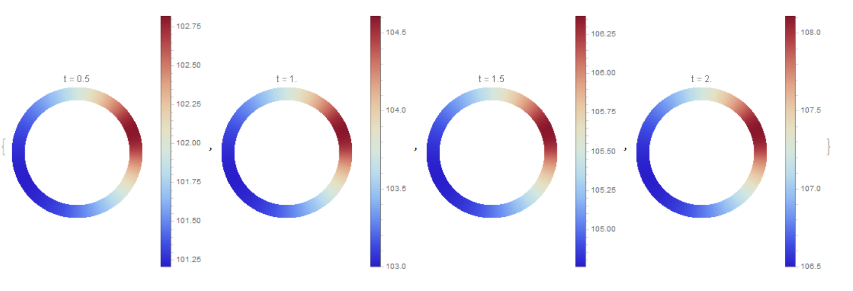
 Also, in version 12, we can use FEM and time dependency. The result completely coincides with that obtained using explicit Euler:
U12 = NDSolveValue[{D[u[t, x, y],
       t] - \[Lambda] Laplacian[
        u[t, x, y], {x, y}] + (x D[u[t, x, y], y] -
        y D[u[t, x, y], x]) - f[ArcTan[x, y]] +
      0.025 (u[t, x, y] - 20) == NeumannValue[10^-9 u[t, x, y], True],
     u[0, x, y] == 100}, u, {t, 0, t1}, {x, y} \[Element] mesh,
   Method -> {"FiniteElement",
     "MeshOptions" -> {"MaxCellMeasure" -> 0.001}}];
Table[DensityPlot[Evaluate[U12[t, x, y]], {x, y} \[Element] mesh,
  PlotLegends -> Automatic, PlotLabel -> Row[{"t = ", t*1.}],
  ColorFunction -> ColorData["ThermometerColors"], PlotPoints -> 100,
  Frame -> False, ColorFunctionScaling -> True, PlotRange -> All], {t,
   10 t0, n*t0, 10 t0}]
The 2D "MethodOfLines" with periodic boundary conditions in polar coordinates gives a solution that does not have physical meaning. For example, the code below has no messages (unlike the one suggested by Ulrich Neumann)
U2 = NDSolveValue[{Derivative[1, 0, 0][u][t, r, \[CurlyPhi]] +
     Derivative[0, 0, 1][u][t,
      r, \[CurlyPhi]] == \[Lambda] Laplacian[
       u[t, r, \[CurlyPhi]], {r, \[CurlyPhi]}, "Polar"] +
     f[\[CurlyPhi]] - 0.025 (u[t, r, \[CurlyPhi]] - 20),
   u[0, r, \[CurlyPhi]] == 100, u[t, r, 0] == u[t, r, 2 Pi],
   Derivative[0, 1, 0][u][t, r1, \[CurlyPhi]] == 0,
   Derivative[0, 1, 0][u][t, r2, \[CurlyPhi]] == 0},
  u, {r, r1, r2}, {\[CurlyPhi], 0, 2 Pi}, {t, 0, t1},
  Method -> {"MethodOfLines",
    "SpatialDiscretization" -> {"TensorProductGrid",
      "MinPoints" -> 40, "MaxPoints" -> 100,
      "DifferenceOrder" -> "Pseudospectral"}}]
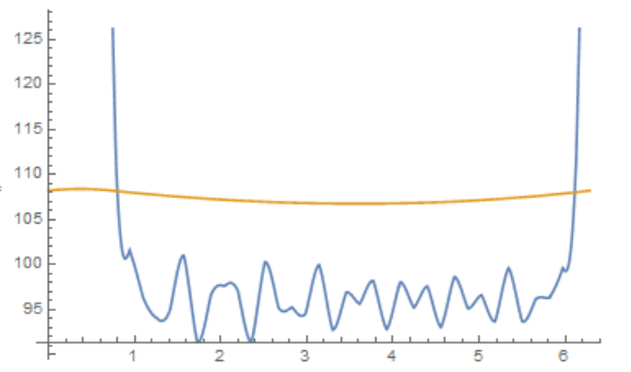
Compare solution U2 and solution U1 (1D "MethodOfLines"). We see that in 2D the heat flux at the boundary $\phi =0=2\pi$ has a gap, which is devoid of physical meaning.
Plot[{U2[2, (r1 + r2)/2, phi], U1[2, phi]}, {phi, 0, 2 Pi}]
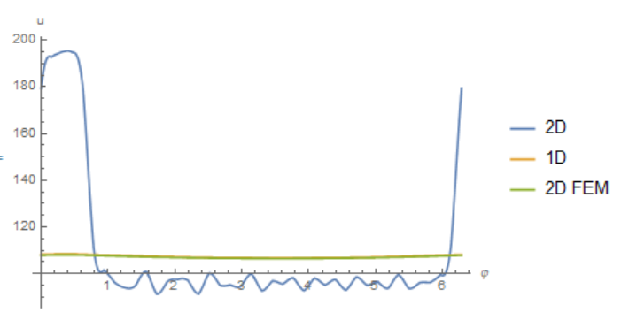
We add the condition of equality of heat fluxes at the boundary $2\pi=\phi =0$. In this case, the solution has the form
U2 = NDSolveValue[{Derivative[1, 0, 0][u][t, r, \[CurlyPhi]] +
     Derivative[0, 0, 1][u][t,
      r, \[CurlyPhi]] == \[Lambda] Laplacian[
       u[t, r, \[CurlyPhi]], {r, \[CurlyPhi]}, "Polar"] +
     f[\[CurlyPhi]] - 0.025 (u[t, r, \[CurlyPhi]] - 20),
   u[0, r, \[CurlyPhi]] == 100, u[t, r, 0] == u[t, r, 2 Pi],
   Derivative[0, 0, 1][u][t, r, 0] ==
    Derivative[0, 0, 1][u][t, r, 2 Pi],
   Derivative[0, 1, 0][u][t, r1, \[CurlyPhi]] == 0,
   Derivative[0, 1, 0][u][t, r2, \[CurlyPhi]] == 0},
  u, {r, r1, r2}, {\[CurlyPhi], 0, 2 Pi}, {t, 0, t1},
  Method -> {"MethodOfLines",
    "SpatialDiscretization" -> {"TensorProductGrid",
      "MinPoints" -> 40, "MaxPoints" -> 100,
      "DifferenceOrder" -> "Pseudospectral"}}]
Now we see an even greater difference between solutions of the equation obtained using 2D "MethodOfLines" and FEM (1D and FEM coincide on this scale).
Plot[{U2[2, (r1 + r2)/2, phi], U1[2, phi],
  U12[2, Cos[phi] (r1 + r2)/2, Sin[phi] (r1 + r2)/2]}, {phi, 0, 2 Pi},
 PlotRange -> All, PlotLegends -> {"2D", "1D", "2D FEM"},
 AxesLabel -> {"\[CurlyPhi]", "u"}]



Derivative[0, 1, 0][u][t, r1, \[CurlyPhi]] == 0, Derivative[0, 1, 0][u][t, r2, \[CurlyPhi]] == 0$\endgroup$TensorPorductGridbyFiniteElementNDSolve doesn't evaluate. Or would you suggest another way? $\endgroup$