Plotting level sets of the form f(x,y,c)==0

Question

I have a problem with making contour plots of the form $f(x,y,c)=0$ work well with Mathematica, where c defines the levelset. For example the lemniscate $(x^2 + y^2)^2 - c (x^2 - y^2) =0$. Obviously rewriting this as $\frac{(x^2 + y^2)^2}{(x^2 - y^2)} =c$ is going to cause some problems for anywhere $x^2=y^2$. If I try to plot multiple curves

ContourPlot[Evaluate@Table[(x^2 + y^2)^2 - m (x^2 - y^2) == 0, {m, 0,4}],
{x, -2, 2}, {y, -2, 2}]

this works but I lose the nice shading in between curves and hover over information about the level sets as seen in this example:

ContourPlot[x^2 + y^2, {x, -2, 2}, {y, -2, 2}]

The best I could do is the following:

lemniscates = 
 Table[
  RegionPlot[{(x^2 + y^2)^2 - m (x^2 - y^2) < 0}, {x, -2, 
     2}, {y, -2, 2}, PerformanceGoal -> "Quality", 
    BoundaryStyle -> None, 
    PlotStyle -> {ColorData[{"RedBlueTones", {0, 7}}][m]}], {m, 0, 
   5}]
Show[Reverse@lemniscates, 
 Prolog -> {ColorData[{"RedBlueTones", {0, 7}}][7], 
   Rectangle[Scaled[{0, 0}], Scaled[{1, 1}]]}]

but this looks awful compared to the default contour plotting and I still lose the level set information. How do I get my lemniscate plots to look like the ContourPlot of the circles example?

Thank you!

EDIT: It seems I used a bit too simple an example with the lemniscates to illustrate my problem. Here is another similar function:

ContourPlot[
 Evaluate@Table[(x^2 + m y^2)^2 - m (x^2 - y^2) == 0, {m, 0, 
    4}], {x, -2, 2}, {y, -2, 2}]

But now solving for m gives you two roots so this will not be easy to put in the required form. What can be done?

Answer 1

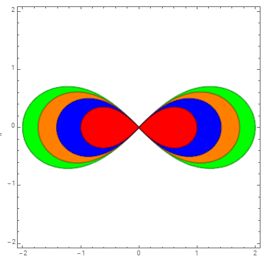
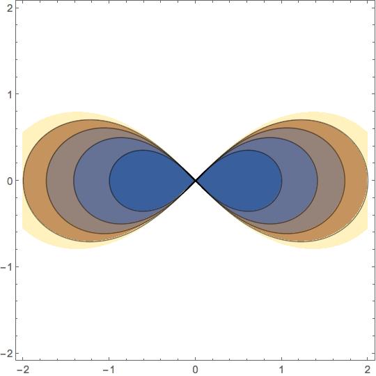
Generate separate ContourPlot for each m with contour 0 and change the tooltip label to m and combine all with Show:

Show @ Table[ContourPlot[Evaluate[(x^2 + y^2)^2 - m (x^2 - y^2)], {x, -2, 2}, {y, -2, 2}, 
    ContourStyle -> Directive[Thick, ColorData[63][m]], 
    ContourShading -> {Opacity[.2, ColorData[63][m]], White}, 
    Contours -> {{0}}] /. Tooltip[a_, _] :> Tooltip[a, m], {m, 0, 4}]

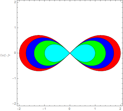
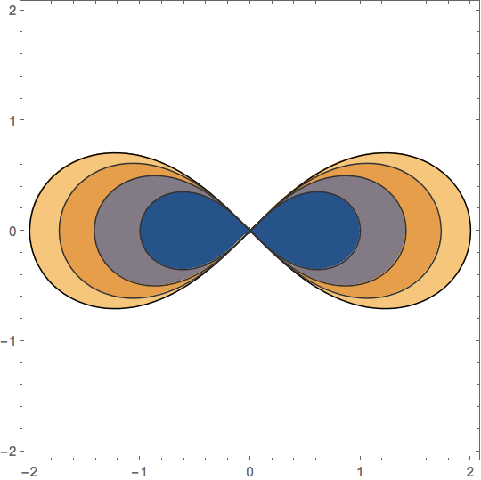
Generate the plots in the opposite order to get opaque colors without blending:

colors = {Cyan, Red, Blue, Orange, Green};
Show @ Table[ContourPlot[(x^2 + y^2)^2 - m (x^2 - y^2) , {x, -2, 2}, {y, -2, 2}, 
    ContourStyle -> Directive[Thick, Darker@Darker@colors[[m + 1]]], 
    ContourShading -> {Opacity[1, colors[[m + 1]]], None}, 
    Contours -> {{0}}] /. Tooltip[a_, _] :> Tooltip[a, m], 
  {m, 4, 0, -1}]

Answer 2

If you can tolerate solving for $1/m$ rather than $m$ (as $m=0$ doesn't given you real numbers), you could use the following:

ContourPlot[(x^2 - y^2)/(x^2 + y^2)^2, {x, -2, 2}, {y, -2, 2},
 Contours -> {1, 1/2, 1/3, 1/4}, PlotRange -> All,
 ContourShading -> {White, Red, Blue, Green, Cyan}]

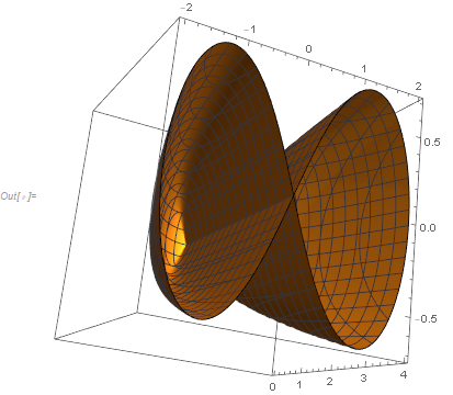
Maybe a more interesting display might be with ContourPlot3D which also allows your actual form of $f(x,y,c)=0$:

ContourPlot3D[(x^2 + y^2)^2 - m (x^2 - y^2) == 0, {x, -2, 2}, {y, -2, 2}, {m, 0, 4}, 
  PlotRange -> All, PlotPoints -> 100]

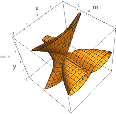
For your more complex example, I think it becomes more important to consider ContourPlot3D:

Answer 3

To get ContourPlot to do what you seek you need to solve for the parameter in the form $m = F(x,y)$; then plot $F(x,y)$ with the desired contours $m$. However, in this OP's case, this causes some numerical problems, which can be alleviated with the following dodge:

ContourPlot[
 (x^2 + y^2)^2/($MachineEpsilon + Abs[x^2 - y^2]),
 {x, -2, 2}, {y, -2, 2},
 Contours -> Table[m, {m, 0, 4}], 
 RegionFunction -> 
  Function[{x, y, z}, x^2 != y^2 && 0 <= (x^2 + y^2)^2/(x^2 - y^2) < 5], 
 MaxRecursion -> 3, PlotPoints -> 25]

Answer 4

This feels somewhat old-school, perhaps because of the expansion of *Plot* functions, I haven't used it in a while. I used to see it used, and used it myself, more often. Basically we project a 3D contour plot of $f(x,y,m)=0$ and project it onto the $xy$-plane.

Like all solutions, it assumes $m$ is a function $m=F(x,y)$ of $x$ and $y$, although unlike my other answer, one does not need to solve for $m$. (If $m$ is not a function of $x$ and $y$, contour regions will overlap where there are multiple values of $m$ for a given $(x,y)$.)

Replace[
 ContourPlot3D[(x^2 + y^2)^2 - m (x^2 - y^2) == 0,
  {x, -2, 2}, {y, -2, 2},
  {m, 0, 4},
  MeshFunctions -> {#3 &}, Mesh -> {Range@4}, 
  MeshShading -> 
   Table[ColorData["M10DefaultDensityGradient"][m/4], {m, 0, 4}],
  PlotPoints -> 35],
 {Graphics3D[dir_, opts___] :>
   Graphics[
    dir /. {GraphicsComplex[pts_, g_, rest___] :>
       GraphicsComplex[
        pts /. {x_Real, y_Real, z_Real} :> {x, y},
        g /. Line[p_] :> Tooltip[Line[p], pts[[First@p, -1]]],
        rest]},
    PlotRange -> 
     Replace[PlotRange /. 
       FilterRules[{opts}, {PlotRange}], {x_, y_, z_} :> {x, y}],
    Frame -> True, Axes -> False,
    FilterRules[{opts}, Options@Graphics]]}
 ]