Plotting the inverse function of a complicated function

Question

So I have a function

F[x_] = Assuming[{Element[x, Reals], -1 < x < 1}, 
           Integrate[1/Sqrt[(x^2 - 1)^2 + alpha*x], x]]

I'm now interested in the inverse function :

G[x_]=InverseFunction[F][x]

But I get no answer from Mathematica...

What I'd like to do is to plot the inverse function, I don't manage to do it... And to play with the values of $\alpha$ please.

Thanks in advance

Answer 1

The antiderivative returned by Integrate has some problems. It might be better to numerically integrate, but take care to avoid the singularity where the square-root is zero:

psol = ParametricNDSolveValue[
    {x'[y] ==  Sqrt[(x[y]^2 - 1)^2 + alpha*x[y]], x[0] == x0,
    WhenEvent[Abs[(x[y]^2 - 1)^2 + alpha*x[y]] < 1*^-6, "StopIntegration"],
    WhenEvent[Abs[x[y]] > xmax, "StopIntegration"]
    }, x, {y, -3, 3}, {alpha, x0, xmax}, 
   Method -> "ExplicitRungeKutta", 
   "ExtrapolationHandler" -> {Indeterminate &}];

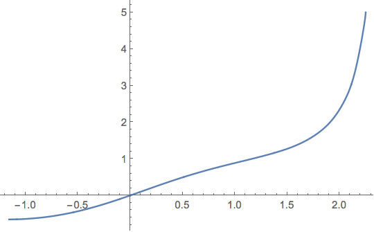
ListLinePlot[psol[0.5, 0, 5], PlotRange -> All, 
 InterpolationOrder -> 3]

Update: Relationship to the OP's Integrate[] result

It's clear that the definite integral $$F(\alpha,x;a)=\int_a^x \frac{1}{\sqrt{\left(\xi^2-1\right)^2+\alpha \xi}} \, d\xi$$ will be real-valued as long as the entire interval $(a,x)$ lies in the region above Root[1 + alpha #1 - 2 #1^2 + #1^4 &, 1] or the region below Root[1 + alpha #1 - 2 #1^2 + #1^4 &, 2]. It should also be clear that over either region, $F$ is monotonic and bounded as a function of $x$. A numerical approximation to the optimal bound may be obtained by setting xmax to the numeric equivalent of infinity, $MaxNumber, in the call to psol above. The bound will be announced in a ParametricNDSolveValue::ndsz error and will depend on the initial condition and alpha. It corresponds to a vertical asymptote in the graph of the inverse function. Similarly the time $y$ to reach the point where the square-root is zero is finite, except for $\alpha = 0$, when the expression under the radical becomes a perfect square.

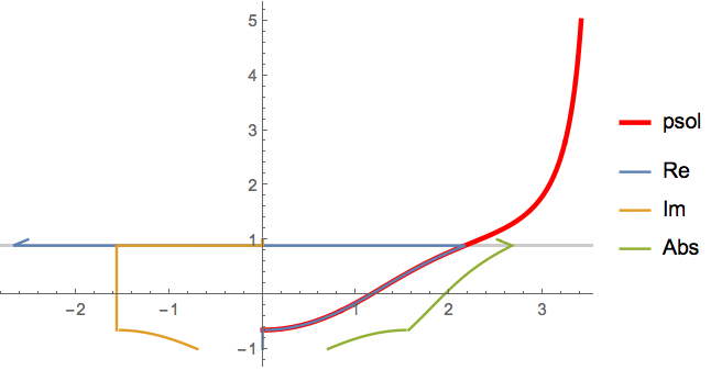
Since any two antiderivatives differ by a constant, the corresponding graphs differ by a translation. The graphs of the inverse functions will differ by a horizontal translation. It's easy to translate the psol solution to overlap the one shown in @BobHanlon's answer for alpha = 0.5:

F[alpha_, x_] =  (* Bob Hanlon's definition *)
  Assuming[{Element[x, Reals], -1 < x < 1}, 
   Integrate[1/Sqrt[(x^2 - 1)^2 + alpha*x], x] // FullSimplify];

p1 = Plot[psol[0.5, 0, 5][x - Re@F[0.5, 0]], {x, -1, 3.5}, 
  PlotStyle -> {AbsoluteThickness[3], Red}, PlotRange -> All,
  PlotLegends -> {"psol"}]

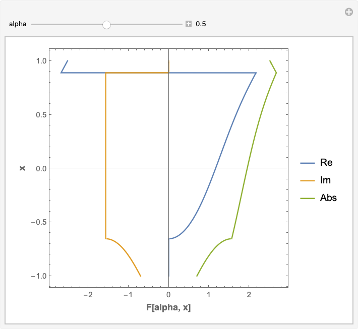
Block[{alpha = 0.5},  (* Bob's plot *)
 p2 = ParametricPlot[
   {{Re@F[alpha, x], x}, {Im@F[alpha, x], x}, {Abs@F[alpha, x], x}},
   {x, -1, 1}, AspectRatio -> 1, 
   PlotRange -> All, Frame -> True, 
   FrameLabel -> (Style[#, 12, Bold] & /@ {"F[alpha, x]", "x"}), 
   PlotLegends -> {Re, Im, Abs}]
 ]

Show[p1, p2, GridLines -> {None, {0.88}}]

Extras

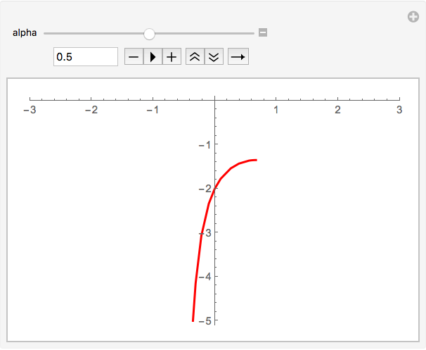
Here's a demo to play with the values of $\alpha$:

Manipulate[
 Quiet@ListLinePlot[psol[alpha, 0, 5], 
   InterpolationOrder -> 3, PlotRange -> {{-3, 3}, {-1.1, 5.1}}],
 {{alpha, 0.5}, 0, 1}]

To play in the other region, change the initial condition parameter x0:

Manipulate[
 Quiet@ListLinePlot[psol[alpha, -2, 5], 
   PlotStyle -> {AbsoluteThickness[2], Red}, InterpolationOrder -> 3, 
   PlotRange -> {{-3, 3}, {-5.1, 0.1}}],
 {{alpha, 0.5}, 0, 1}]

Answer 2

Inverse functions can be plotted using ParametricPlot or ParametricPlot3D

Clear["Global`*"]

F[alpha_, x_] = 
  Assuming[{Element[x, Reals], -1 < x < 1}, 
   Integrate[1/Sqrt[(x^2 - 1)^2 + alpha*x], x] // FullSimplify];

Manipulate[
 ParametricPlot[{
    {Re@F[alpha, x], x},
    {Im@F[alpha, x], x},
    {Abs@F[alpha, x], x}},
   {x, -1, 1},
   AspectRatio -> 1,
   PlotRange -> All,
   Frame -> True,
   FrameLabel -> (Style[#, 12, Bold] & /@ {"F[alpha, x]", "x"}),
   PlotLegends -> {Re, Im, Abs}] //
  Quiet,
 {{alpha, 0.5}, 0.005, 1, 0.005, Appearance -> "Labeled"}]