This answer addresses some of your question, which is actually fairly broad and I think touches as much on the underlying concepts as on how to use Mathematica to achieve the stated goal.
This will answer:
- How to import a wav file as samples
- How to get the discrete Fourier transform normalized to give expected magnitudes
- How to get a range of frequencies
- How to get the magnitudes at those frequencies
Step 1: Import the wav file as samples:
signal = First@Import["D:\\audio\\Airwolf.wav", "Data"]
Here I use First to get just one stereo channel. Use "Elements" instead of "Data" above to reveal other options to pass as the 2nd argument to Import to find (for example) how many channels there are and what the sampling rate is.
You can test your techniques by using a sampled sine, rather than a wav file, where you control the magnitude, frequency, and phase. This generates 1 second of a 440Hz sine with magnitude 1 and zero phase shift:
Table[Sin[2 Pi t 440], {t, 0, 1, 1./10000}]
Step 2: Use the Fourier function to get the discrete Fourier transform:
dft=Fourier[signal, FourierParameters -> {-1, 1}]
I use FourierParameters -> {-1,1} to get magnitudes that you expect from the symbolic Fourier transform. For example, if signal was sampled from a 440Hz sine wave with magnitude k:
$$f(t) = k * sin(2 \pi 440 t)$$
then the symbolic Fourier transform will give a Dirac delta at +/-440Hz with magnitude k/2, and FourierParameters->{-1,1} will give the same magnitudes. Read the docs for more info. The default option value normalizes the magnitudes differently.
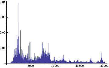
You can plot the audible portion of this:
ListLinePlot[Part[dft, 1 ;; 20000], PlotRange -> Full]

Step 3: Get a range of frequencies from 101 to 200 Hz:
range = Part[dft, 101;;200]
Step 4: Get their magnitudes with the Abs function:
mag = Abs[range]
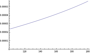
You can plot the magnitudes for this range:
ListLinePlot[Transpose[{Range[101, 200], mag}], PlotRange -> Full]


