plot line, combine graphics and Plot in Maxwell distribution

Question

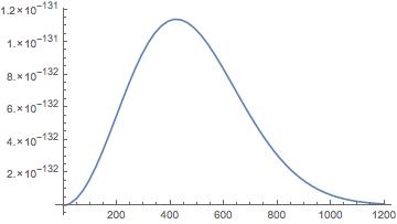
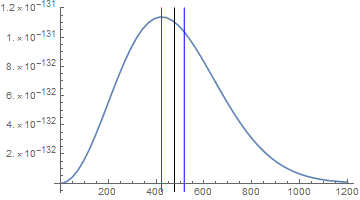
i'm trying to plot Maxwell distribution and draw a line where average speed varg, most probable speed vm, and rms speed vrms, and label those lines.

my struggle how to plot these lines and combine graphics with plot in Show.

here is the code easy and short!

k = 1.38064852*10^(-23);
m = 28*1.660538782*10^(-27);
t = 300;

max[v_] := ((m/2 Pi k t)^3/2 )*(4 Pi v^2) Exp[-((m*v^2)/(2 k t))]


p1 = Plot[max[v], {v, 0, 1200}]

vm = Sqrt[2 k t/m]
vrms = Sqrt[3 k t/ m]
vavg = Sqrt[8/Pi]*Sqrt[k t /m]

l1 = Graphics[Line[{vm, 0}, {vm, y}]]
l2 = Line[{0, vrms}]
l3 = Line[{0, vavg}]

Show[p1, l1]

Answer 1

With your definitions, consider something like this:

l1 = InfiniteLine[{{#, 0}, {#, 1}}] &[vm];
l2 = InfiniteLine[{{#, 0}, {#, 1}}] &[vrms];
l3 = InfiniteLine[{{#, 0}, {#, 1}}] &[vavg];

Show[
 p1,
 Graphics[{Red, l1, Blue, l2, Black, l3}]
]

Answer 2

Your definition for max is not a valid PDF

max[v_] := ((m/2 Pi k t)^3/2)*(4 Pi v^2) Exp[-((m*v^2)/(2 k t))]

The total probability should be 1

Assuming[m > 0 && k > 0 && t > 0,
 Integrate[max[v], {v, 0, Infinity}]]

(* (m^(3/2) π^(9/2) (k t)^(9/2))/(4 Sqrt[2]) *)

You probably intended to use

max[v_] := (m/(2 Pi k t))^(3/2)*(4 Pi v^2) Exp[-((m*v^2)/(2 k t))]

This is a valid PDF

Assuming[m > 0 && k > 0 && t > 0,
 Integrate[max[v], {v, 0, Infinity}]]

(* 1 *)

You would be better off using the built-in MaxwellDistribution

dist = MaxwellDistribution[Sqrt[k t/m]];

This has the same PDF as the revised max

Assuming[m > 0 && k > 0 && t > 0 && v > 0,
 PDF[dist, v] == max[v] // Simplify]

(* True *)

vavg = Mean[dist]

(* 2 Sqrt[2/π] Sqrt[(k t)/m] *)

vrms = RootMeanSquare[dist]

(* Sqrt[3] Sqrt[(k t)/m] *)

The mode is

vm = v /. Solve[{D[PDF[dist, v], v] == 0 && 
    m > 0 && k > 0 && t > 0 && v > 0}, v][[1]] // 
  Simplify[#, m > 0 && k > 0 && t > 0] &

(* Sqrt[2] Sqrt[(k t)/m] *)