Error propagation in finding full width at half maximum

Question

I have an equation given by:

f[x_,M_]:= 96.4529 E^(M x (-0.216331 - 38.7396 M x)) + 31.0508 E^(M x (0.306405 - 18.585 M x)) + 4.36041 E^(M x (3.95974 - 7.37814 M x)) + 2.00366 E^(M x (-1.54639 - 3.79704 M x)) + 119.8 E^(M x (-0.0235058 - 0.0245919 M x));

where $x$ is a variable, $M$ is the mean value from a measurement and $\delta M$ is the error in $M$. For example, let $M \pm \delta M$ be equal to $ 15.584 \pm 0.045$.

The approximate error $\delta f$ in $f$ can be given, in the simplified form assuming indipendence of $x$ and $M$, as:

$$\delta f = \sqrt{\left(\frac{\partial f}{\partial M}\right)^2(\delta M)^2 + \left(\frac{\partial f}{\partial x}\right)^2(\delta x)^2}$$

As $x$ is not a measured value, I take $\delta x = 0$ :

DfM[x_, M_] := Evaluate@ D[f[x, M], M];
Dfx[x_, M_] := Evaluate@ D[f[x, M], x];
Deltaf[x_, M_, deltaM_] := Evaluate@ Simplify[Sqrt[(DfM[x, M])^2 deltaM^2 
                                       + (Dfx[x, M])^2 deltax^2]] /. {deltax -> 0};

This way I can find the error $\delta f$ in $f$ that is a consequence of the error $\delta M$ in $M$.

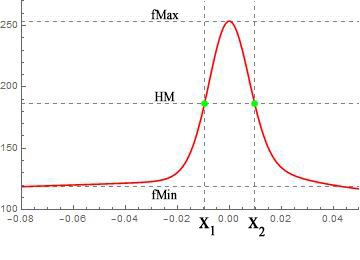
But my aim is to find the full width at half maximum (FWHM) i.e. $$FWHM \pm \delta FWHM = (x_2-x_1) \pm \sqrt{(\delta x_1)^2 + (\delta x_2)^2}$$ along with the error $\delta FWHM$ that propagates in doing so. Here, $x_1$ and $x_2$ are the corresponding $x$-axis values for the half maximum HM. The errors in $x_1$ and $x_2$ are $\delta x_1$ and $\delta x_2$, respectively.

To find the half of the maximum (i.e. HM) , I find the maxima and minima of f[x,M] as:

fMin = First[NMinimize[{f[x, 15], -0.08 < x < 0.04}, x]];
fMax = First[NMaximize[f[x, 15], x]]; 
HM = fMax + (fMin - fMax)/2;  

There will be some error in HM i.e. $\delta HM$ but I am unable to figure out how this error is propagating via the NMaximize and NMinimize functions. Additionally, to find the $x_1$ and $x_2$ I need to solve the function f[x,M] for the value HM but this function does not seem to have an inverse and therefore Solve fails if I use:

Solve[f[x, 15] == HM, x]

Is there a way I could find $FWHM$ and its error $\delta FWHM$?.

EDIT:

Link to the data of which fun[x] is a nonlinear fit: Data

fun[x_] := 96.4529 E^((-0.216331 - 38.7396 x) x) + 31.0508 E^((0.306405 - 18.585 x) x) +  4.36041 E^((3.95974 - 7.37814 x) x) +  2.00366 E^((-1.54639 - 3.79704 x) x) +  119.8 E^((-0.0235058 - 0.0245919 x) x);

the function f[x_,M_] given above is derived using fun[x_] as:

f[x_,M_] := fun[x*M];

Answer 1

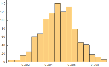
Here is a bootstrap approach to estimate a standard error associated with the estimate of $x_2-x_1$.

data = {{-1.5, 117.955}, {-1.452, 118.277}, {-1.404, 119.012}, {-1.356, 119.277}, 
  {-1.308, 120.204}, {-1.26, 120.545}, {-1.212, 120.866}, {-1.164, 120.712},
  {-1.116, 120.37}, {-1.068, 120.523}, {-1.02, 120.848}, {-0.972, 120.798},
  {-0.924, 120.98}, {-0.876, 121.441}, {-0.828, 121.496}, {-0.78, 121.163},
  {-0.732, 120.515}, {-0.684, 121.504}, {-0.636, 121.139}, {-0.588, 119.96},
  {-0.54, 119.393}, {-0.492, 120.752}, {-0.444, 122.253}, {-0.396, 123.639},
  {-0.348, 126.277}, {-0.3, 131.765}, {-0.252, 139.704}, {-0.204, 154.437},
  {-0.156, 180.332}, {-0.108, 214.055}, {-0.06, 242.769}, {-0.012, 255.787},
  {0.036, 249.115}, {0.084, 224.131}, {0.132, 194.485}, {0.18, 171.191},
  {0.228, 155.534}, {0.276, 143.708}, {0.324, 134.348}, {0.372, 129.606},
  {0.42, 127.123}, {0.468, 124.993}, {0.516, 122.399}, {0.564, 120.834},
  {0.612, 120.375}, {0.66, 119.378}, {0.708, 118.306}, {0.756, 116.853},
  {0.804, 115.839}};

Now the function to be fit:

f[x_, a1_, b1_, c1_, a2_, b2_, c2_, a3_, b3_, c3_, a4_, b4_, c4_] :=
  a1 E^(x (b1 + c1 x)) +
  a2 E^(x (b2 + c2 x)) +
  a3 E^(x (b3 + c3 x)) +
  a4 E^(x (b4 + c4 x));

(* Initial parameter values *)
inits = {
   {a1, 55}, {b1, 1}, {c1, -20},
   {a2, 20}, {b2, 2}, {c2, -1},
   {a3, 12}, {b3, -1.5}, {c3, -53},
   {a4, 120}, {b4, -0.5}, {c4 , -0.2}};

findx1x2[data_] := 
 Module[{nlm, fmax, fmin, HM, x1, x2, xfmax, xfmin, x2Init},
  nlm = NonlinearModelFit[data, f[x, a1 , b1 , c1 , a2 , b2 , c2 , a3 , b3, c3, a4 , b4, c4], 
    inits, x, MaxIterations -> 1000];
  fmax = FindMaximum[nlm[x], {x, Select[data, #[[2]] == Max[data[[All, 2]]] &][[1, 1]]}];
  fmin = FindMinimum[{nlm[x], -1.5 < x < 0.8}, {x, Select[data, #[[2]] == Min[data[[All, 2]]] &][[1, 1]]}];
  xfmax = x /. fmax[[2]];
  xfmin = x /. fmin[[2]];   
  HM = (fmin[[1]] + fmax[[1]])/2;
  x1 = x /. FindRoot[nlm[x] == HM, {x, (x /. fmax[[2]])}];
  x2Init = If[x1 < xfmax, xfmax + (xfmax - x1), xfmax + (xfmax - x1)];
  x2 = x /. FindRoot[nlm[x] == HM, {x, x2Init}];
  {Min[x1, x2], Max[x1, x2], HM, fmin[[1]], fmax[[1]]}]

The bootstrap process (random selection of residuals):

(* Get predicted responses and fit residuals *)
nlm = NonlinearModelFit[data, 
   f[x, a1 , b1 , c1 , a2 , b2 , c2 , a3 , b3, c3, a4 , b4, c4], 
   inits, x, MaxIterations -> 1000];
predictedResponse = nlm["PredictedResponse"];
fitResiduals = nlm["FitResiduals"];

(* Array to hold bootstrap estimates *)
nboot = 1000;
x1x2 = ConstantArray[{0, 0, 0, 0, 0}, nboot];

(* Perform bootstraps *)
n = Length[data];
SeedRandom[12345];
Do[
 boot = Transpose[{data[[All, 1]], predictedResponse + RandomChoice[fitResiduals, n]}];
 x1x2[[iboot]] = findx1x2[boot],
 {iboot, nboot}]

(* Summarize results *)
mle = findx1x2[data]
(* Estimate of x2 - x1 *)
estimate = mle[[2]] - mle[[1]]
(* 0.29482173864942085 *)
(* Standard error of x2 - x1 *)
stderr = StandardDeviation[x1x2[[All, 2]] - x1x2[[All, 1]]]
(* 0.0014648255351604935 *)

(* Histogram of bootstrap estimates *)
Histogram[x1x2[[All, 2]] - x1x2[[All, 1]]]

Edit

If the quantity of interest is $(x_2-x_1)/M$, then applying the Propagation of Error (Delta) method results in an estimate of the variance as

$$\frac{\sigma_M^2 (x_2-x_1)^2}{M^4}+\frac{\sigma_{x_2-x_1}^2}{M^2}$$

assuming that the estimate of $x_2-x_1$ is statistically independent from the estimate of $M$. So we have

results = {x1 -> mle[[1]], x2 -> mle[[2]], σx1x2 -> stderr, M -> 15.584, σM -> 0.045}
estimate = (-x1 + x2)/M /. results
(* 0.0189182 *)
seEstimate = (σx1x2^2/M^2 + σM^2 (x2 - x1)^2/M^4)^0.5 /. results
(* 0.000108717 *)

Answer 2

This is an extended comment rather than an answer.

While I still think that a bootstrap approach would be more accurate than using the Propagation of Error/Delta Method, there are two issues you might want to consider first.

1. The parameter correlation matrix for your current model suggests that using 5 kernels is way overfitting (with $a_i e^{M x(b_i+c_i M x)}$ being a kernel). Fitting a model with just 4 kernels has a much smaller AIC (Akaike Information Criterion) and fits almost perfectly with no errors.

2. If you are after predictions or making inferences about $x_1$ and $x_2$, $M$ is completely irrelevant because $M$ and $x$ always appear together as a product with an associated coefficient.

   More specifically the kernel $a e^{M x(b+c M x)}$ results in the same prediction as $a e^{x(B+C x)}$. (If $M$ appeared away from $x$, then that would be a different story.)