Estimation of the error for zero degree of freedom fit with error bar

Question

I am performing a fit on experimental data with zero degree of freedom but with error bar using NonlinearModelFit:

nlmSimple = NonlinearModelFit[p[[All, 1]], a*Exp[-t/k1], {{a, 3000}, {k1, 600}},   t, Weights -> 1/p[[All, 2, 1]]^2,    VarianceEstimatorFunction -> (1 &), MaxIterations -> 200];

where p[[All, 1]]=$\{\{x1,y1\},\{x2,y2\}\}$ is a couple of data point and p[[All, 2, 1]] the associated error on $y_i$ ( which is basically the square-root of the experimental data).

Of course residuals are zero since degree of freedom is zero (=> the function take exactly the value of the data). Consequences : all the standard tools for errors estimations, confidence level etc. of Mathematica are not working.

But I should be able to extract an error since the errors I am using are not equal to zero.

Is there any Mathematica function/option/argument for doing this or I have to build my own tool (and go through the maths... ) ?

Thank you for your help

edit :

The data are describe the radiocative decay of particles. $x_i$ is the number of surviving particle.

So that mean my $x_i$ folllow the binomiale distribution : $\binom{a}{k} p^k(1-p)^{n-k}$ with $p= exp(-y_i/k1)$.

As in practice $x_i>1000$ is quite large and $p \in [ 0.05, 0.9] $ the distribution of $x_i$ convergence toward normal distribution.

Answer 1

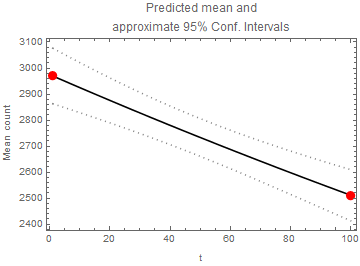
Additional edit: I showed how to obtain standard errors for the parameters but maybe what you mean by "estimation of the error" is a confidence interval for the mean prediction. I've added that below. (If you need 95% prediction intervals, then those would be much wider.)

Edit: With the additional information given in the question, it seems clear that you need to perform a Poisson regression.

It appears that you have two counts of particles each over a different length of time. In the olden days one would take the square root of the count and perform a standard linear regression as the square root transformation stabilizes the variance of Poisson counts.

But in the last 20 years or so that's no longer necessary. Software is readily available to explicitly recognize the integral role of the Poisson distribution. Mathematica has GeneralizedLinearModelFit to do so. (It would be even nicer if Mathematica had GeneralizedLinearMixedModelFit but that might have to wait until version 14.)

The model set-up would be the following:

$$y_i \sim Poisson(\lambda_i)$$

$$\log(\lambda_i)=c_0+c_1 t_i$$

Using your notation $\log(\lambda_i)=\log(a)-t_i/k_1$ so GeneralizedLinearModelFit estimates $c_0=\log(a)$ and $c_1=-1/k_1$. To get estimates of the standard errors of the estimators of $a$ and $k_1$ we'll need to use the Delta Method (a.k.a Propagation of Error method).

(* Set parameters *)
a = 3000;
k1 = 600;

(* Generate two data points where y ~ Poisson(a Exp[-t/k1]) *)
t = {1, 100};  (* Lengths of time *)
SeedRandom[12345];
y = Flatten[RandomVariate[PoissonDistribution[a Exp[-#/k1]], 1] & /@ t]
data = Transpose[{t, y}]

(* Perform a Poisson regression *)
(* y ~ Poisson(λ_t) *)
(* log(λ_t)= c0 + c1 t *)
(* where c0 = Log[a] and c1 = -1/k1 *)
(* This is equivalent to y ~ Poisson(a Exp[-t/k1]) *)
glm = GeneralizedLinearModelFit[data, z, z, ExponentialFamily -> "Poisson"];

(* Get parameter estimates which are estimates of Log[a] and 1/k1 *)
{loga, minusRecipk1} = glm["BestFitParameters"];
(* Estimates of a and k1 from Poisson regression *)
ahat = Exp[loga]
(* 2924.6191888146855 *)
k1hat = -1/minusRecipk1
(* 807.5868297019861 *)

Note that we can get the estimates directly without having to run GeneralizeLinearModelFit:

(* Estimate of a *)
N[y[[1]] (y[[1]]/y[[2]])^(1/(t[[2]] - t[[1]]))]
(* 2924.6191888146923 *)

(* Estimate of k1 *)
N[(t[[2]] - t[[1]])/Log[y[[1]]/y[[2]]]]
(* 807.5868297019673 *)

But we need to run GeneralizedLinearModelFit to get the estimate of the parameter covariance matrix. (Although this could be more directly estimated using LogLikelihood.)

Using the Delta Method one can obtain estimates of the standard errors of ahat and k1hat:

covGLM = glm["CovarianceMatrix"];
seahat = Exp[loga] covGLM[[1, 1]]^0.5
(* 54.662928826594296 *)
sek1hat = (1/minusRecipk1^2) covGLM[[2, 2]]^0.5
(* 177.91390393430407 *)

To obtain approximate confidence intervals for the mean prediction we'll also need to use the Delta method.

se[z_, cov_, mle_] := 
  (D[Exp[c0 + c1 z], {{c0, c1}}].cov.D[Exp[c0 + c1 z], {{c0, c1}}] /. 
  {c0 -> mle[[1]], c1 -> mle[[2]]})^0.5

For this particular sample the standard error for a particular time length $t$ is

$$\left(e^{-0.00338036 t} ((0.673417 t-62.4452) t+3086.14)\right)^{0.5}$$

Show the prediction and confidence intervals:

Show[Plot[{glm[z], glm[z] + 1.96 se[z, covGLM, {loga, minusRecipk1}],
  glm[z] - 1.96 se[z, covGLM, {loga, minusRecipk1}]}, {z, t[[1]], t[[2]]},
  PlotStyle -> {Black, {Dotted, Gray}, {Dotted, Gray}}, Frame -> True,
  FrameLabel -> {"t", "Mean count"},
  PlotLabel -> "Predicted mean and\napproximate 95% Conf. Intervals"],
 ListPlot[data, PlotStyle -> {{Red, PointSize[0.03]}}]]

The estimates of the standard errors at $t_1$ and $t_2$ work out to be simply $\sqrt{y_1}$ and $\sqrt{y_2}$, respectively.