Use of GPU/CUDA to speed up rendering of surface

Question

I am attempting to create several surface renderings of expressions that come out of a solution for the eigenvalues of a matrix and the resulting expressions are considerably messy

The eigenvalue functions end up looking like this

Fcoupleda = -z + Root[-187.25 + 80.75 x^2 - 4. x^4 - 1. x^6 + 109.119 y - 
 55.4256 x^2 y + 6.9282 x^4 y - 111.25 y^2 - 24. x^2 y^2 - 
 3. x^4 y^2 + 55.4256 y^3 + 13.8564 x^2 y^3 - 20. y^4 - 
 3. x^2 y^4 + 6.9282 y^5 - 
 1. y^6 + (111.25 + 24. x^2 + 3. x^4 - 55.4256 y - 
    13.8564 x^2 y + 40. y^2 + 6. x^2 y^2 - 13.8564 y^3 + 
    3. y^4) #1 + (-20. - 3. x^2 + 6.9282 y - 3. y^2) #1^2 + 
 1. #1^3 &, 1] == 0

And the plot code is

plotcoupled = ContourPlot3D[Evaluate[Fcoupleda], {x, -6, 6}, {y, -4, 7}, {z, 0, 15}, AxesLabel -> {x, y, z}]

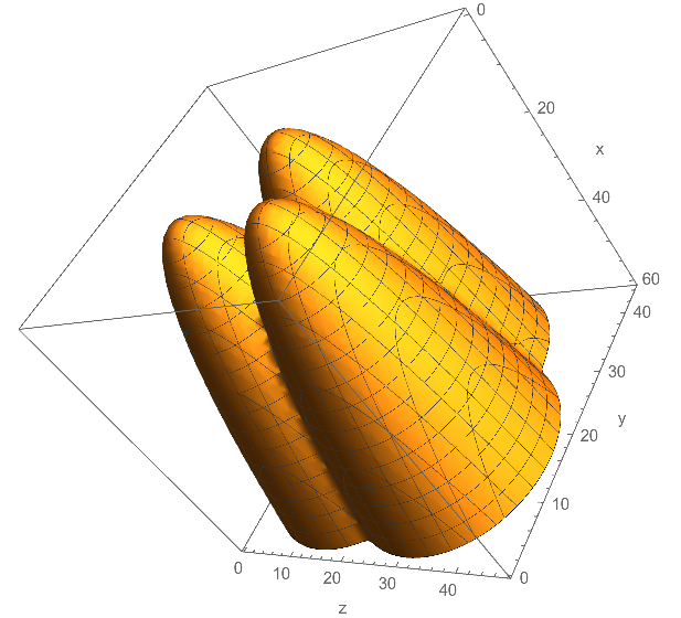
Understandably, when i try to plot these using contourplot3d with a decent point count it takes way too long to come up with a reasonably high quality graph. Does anyone know a good way to put the evaluation of the expression over the variables onto a GPU and still end up with a similar looking surface plot to contourplot3d? I have a 980ti and would love to just dump the calculations onto the GPU

Answer 1

This might be a bit faster although it does not look as fancy as output of ContourPlot3D. It needs 4 seconds on my laptop:

f = -z + Root[-187.25 + 80.75 x^2 - 4. x^4 - 1. x^6 + 109.119 y - 
      55.4256 x^2 y + 6.9282 x^4 y - 111.25 y^2 - 24. x^2 y^2 - 
      3. x^4 y^2 + 55.4256 y^3 + 13.8564 x^2 y^3 - 20. y^4 - 
      3. x^2 y^4 + 6.9282 y^5 - 
      1. y^6 + (111.25 + 24. x^2 + 3. x^4 - 55.4256 y - 
         13.8564 x^2 y + 40. y^2 + 6. x^2 y^2 - 13.8564 y^3 + 
         3. y^4) #1 + (-20. - 3. x^2 + 6.9282 y - 3. y^2) #1^2 + 
      1. #1^3 &, 1];
dx = 0.25;
dy = 0.25;
dz = 0.25;
data = ParallelTable[
     f, 
     {x, -6., 6., dx}, 
     {y, -4., 7., dy}, 
     {z, 0., 15., dz}
     ]; // AbsoluteTiming // First

ListContourPlot3D[data, Contours -> {0.}, AxesLabel -> {"x", "y", "z"}]

4.08582