Your problem is similar to a wave spectra problem and a regression problem, and I have both types of problems going on at work right now which is why I've thought about your problem a bit.
Here is an approach with bootstrapping. I used FourierDCT because I don't want to figure out the circular statistics of complex numbers...
bootStrapUDList[listFuncHead_,data_]:=PlusMinus@@@MapThread[Through[{Mean,(Max@#-Min@#)/2&}@{##}]&,MapThread[listFuncHead[{##}]&,data/.pm_PlusMinus:>RandomVariate[UniformDistribution@Sort@{Subtract@@pm,Plus@@pm},200000]]]

bootStrapNDList[listFuncHead_,data_]:=PlusMinus@@@MapThread[Through[{Mean,StandardDeviation}@{##}]&,MapThread[listFuncHead[{##}]&,data/.pm_PlusMinus:>RandomVariate[NormalDistribution@@pm,200000]]]

Short[InputForm[data=Table[PlusMinus[Sin[2\[Pi] t]+RandomReal[{-10^-3,10^-3}],10^-3+10^-2t],{t,0,2,0.01}]],5]
(*{-0.00015902041160618116 ± 0.001, 0.06369389709857176 ± 0.0011, 0.12615800788307047 ± 0.0012000000000000001, 0.18766842577245152 ± 0.0013, 0.24919853862147867 ± 0.0014, <<193>>, -0.12457700878215405 ± <<1>>, -0.06205334281024041 ± 0.020900000000000002, 0.0009467025819242354 ± 0.021}*)

(*dctData is the data you're asking about in your question, but I don't plot it directly
here*)
Short[InputForm[dctData=bootStrapNDList[FourierDCT,data]],5]
(*{-0.00013058978084242337 ± 0.01243461722327339, 2.3922514484284694 ± 0.009345519847128744, 0.0004364938928370489 ± 0.008935073841291516, 5.06557192629556 ± 0.008842253876933912, <<195>>, 0.0003672953018113705 ± 0.008634731807823369, 0.0007823963956902927 ± 0.008202728384246478}*)

Short[InputForm[invDCTData=bootStrapNDList[FourierDCT[#,3]&,dctData]],5]
(*{-0.0001489981017240066 ± 0.012484433568524647, 0.06363813654805517 ± 0.012452403598913883, 0.1261974349932789 ± 0.012437140396949981, 0.18770987190793406 ± 0.012447580994827578, <<195>>, -0.062018564059908 ± 0.012431168492616582, 0.0010387203700553621 ± 0.012455374980166786}*)

ListPlot[#,PlotMarkers->Automatic]&/@Outer[#1/@#2&,{First,Last},{data,invDCTData},1]

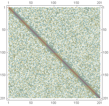
dctData is the data you're asking about in your question, but I don't plot it directly here. In the 2nd graphic, where we show uncertainties from the inverse Fourier-transform, I think the uncertainties don't match the original because the 2nd bootstrap starts from the already Fourier-transformed data and assumes that the uncertainties in the coefficients are uncorrelated. However, we can show that the Fourier coefficients are correlated with each other. You will need to take this into account if you do subsequent calculations with dctData. Lack of correlation tracking is also the reason why precision tracking can't be used for uncertainty analysis.
Correlation[MapThread[FourierDCT[{##}]&,data/.pm_PlusMinus:>RandomVariate[NormalDistribution@@pm,20000]]];
Length@Cases[%,x_?NumericQ/;Abs@x>.25,Infinity]
MatrixPlot@%%
(*601*)
In order to show the uncertanties on top of each other, you would have to issue:
invDCTData=bootStrapNDList[FourierDCT[FourierDCT@#,3]&,data]]
But that would be rather boring.
I also wrote a package to do uncertainty tracking a long time ago. I don't know if it works now.
Here is an example of its output.
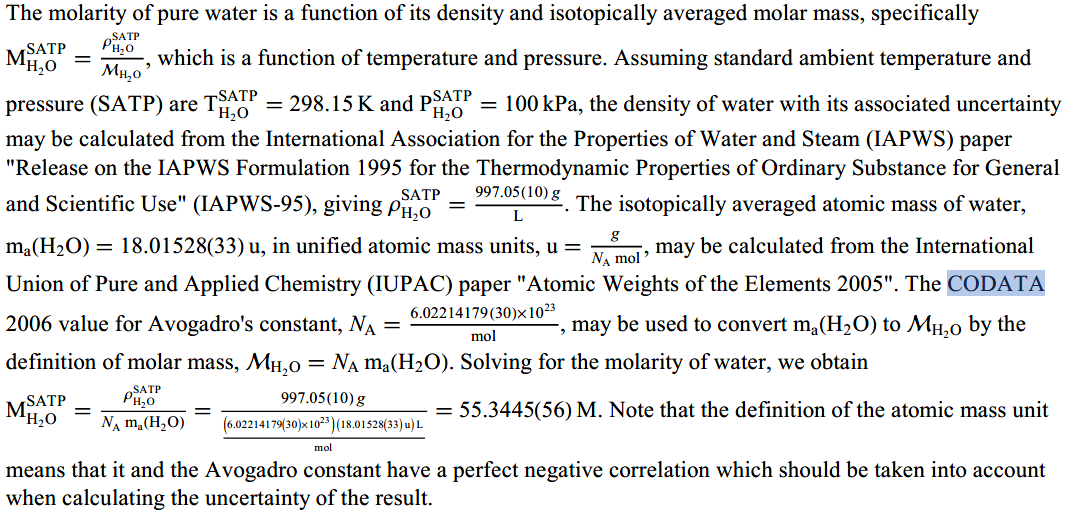
All of the functions and objects mentioned below have help text, which you can read in the package or on which you can use ? (Information).
Here are some of the simpler functions the package defines.
StringToUncertainNumber defines a regular number with an uncertainty, returning an UncertainNumber object. SetCorrelationCoefficient allows manual flagging of numbers that you know to be correlated.

PropagateUncertainty returns a new UncertainNumber object with the correct correlations to the UncertainNumber objects that comprise it. I think I designed it to work even if the number or its uncertainty is symbolic.

The package structure should be a single folder called Uncertainty with Uncertainty.m and the Kernel folder. Inside the Uncertainty\Kernel, an init.m file is needed with just two lines of content:
(* ::Package:: *)

Get["Uncertainty`Uncertainty`"]
Here is the program listing (pacakge) for Uncertainty.m. There are some simple examples (but no output) at the end. If you are wondering why it is called Uncertainty instead of error or standard deviation, it reflects the terminology in the ISO Guide to the Expression of Uncertainty in Measurement. The central algorithm works by maintaining a dynamic list of unique symbols that track correlations (or the lack thereof) and using an associated generalized matrix of correlation coefficients.
(* ::Package:: *)

BeginPackage["Uncertainty`"]
(* Exported symbols added here with SymbolName::usage *)


MakeUncertainNumber::"usage"="MakeUncertainNumber[est,unc] creates a new UncertainNumber object with an estimate of est and an uncertainty of \
unc. MakeUncertainNumber[var,est,unc] creates an uncertain number object, but allows you to specify the symbol, var, with which est and unc are \
associated.";


CorrelationCoefficient::"usage"="CorrelationCoefficient[unc1,unc2] gives the correlation coefficient between two uncertain numbers, \
unc1 and unc2.";


SetCorrelationCoefficient::"usage"="SetCorrelationCoefficient[unc1,unc2,val] assigns a correlation coefficient between two uncertain \
numbers, unc1 and unc2. val should be between -1 and 1, inclusive.";


UnsetCorrelationCoefficient::"usage"="UnsetCorrelationCoefficient[unc1,unc2] removes a correlation coefficient between two uncertain \
numbers, unc1 and unc2.";


StringToUncertainNumber::"usage"="StringToUncertainNumber[str] returns the UncertainNumber object representing str. For instance \
StringToUncertainNumber[\"1.234(56)\"] will return an expression that looks like UncertainNumber[1.234,0.056,symb] in StandardForm, \
where symb is a unique tracking symbol. In FullForm, the returned expression is actually UncertainNumber[symb]. In TraditionalForm, \
the representation is 1.234(56).";


Uncertainty::"usage"="Uncertainty[symb] gives the uncertainty of symb. If an UncertainNumber object is supplied, symb is extracted from that.";


Estimate::"usage"="Estimate[symb] gives the estimate of symb. If an UncertainNumber object is supplied, symb is extracted from that.";


UncertainNumber::"usage"="UncertainNumber[symb] represents an uncertain number, tracked by the symbol symb, which is typically thought of as \
a two parameter statistical distribution with an expectation and standard deviation. However, there is often not enough evidence to justify \
actually calling an uncertain number a distribution, so we refer to the expectation as an estimate and the standard deviation as the \
uncertainty. By using linear properties of the covariance operator, functions of uncertain numbers may, in turn, have their own uncertainties \
evaluated and be turned into new UncertainNumber objects. This is sometimes called the \"law\" of propagation of error (or uncertainty). See \
the usage message for StringToUncertainNumber for a description of the different printed formats of an UncertainNumber object.";


PropagateUncertainty::"usage"="PropagateUncertainty[expr] attempts to propagate uncertainty via UncertainNumber objects using a first \
order approximation to the deviation from the expected value of expr. All unique uncertain numbers are treated as uncorrelated unless \
specified by via SetCorrelationCoefficient. The result of this command is a new unique UncertainNumber object.";


UncertainNumberToNormal::"usage"="UncertainNumberToNormal[expr] converts uncertain numbers within expr to their estimates.";


Begin["`Private`"]
(* Implementation of the package *)


newUncertainNumberSymbol[]:=Module[{var},var]

MakeUncertainNumber[est_,unc_]:=MakeUncertainNumber[newUncertainNumberSymbol[],est,unc]

MakeUncertainNumber[var_,est_,unc_]:=
    (var/:Estimate[var]=est;
    var/:Uncertainty[var]=unc;
    UncertainNumber[var])


(*Estimate and Uncertainty operate on the unique symbols we use to track uncertainty*)
(#[UncertainNumber[var_]]:=#@var)&/@{Estimate,Uncertainty}


UncertainNumber/:Normal[UncertainNumber[var_]]:=Estimate@var

UncertainNumberToNormal[xpr_]:=xpr/.unc_UncertainNumber:>Normal@unc;


StringToUncertainNumber[str_String]:=MakeUncertainNumber@@
    StringReplace[str,
        StringExpression[first__?DigitQ,".",second__?DigitQ,"(",uncert__?DigitQ,")"]:>
            ToExpression[first<>"."<>second,InputForm]~~
                ToExpression[StringJoin["0.",Table["0",{StringLength@second-StringLength@uncert}],uncert],InputForm]
        ]


getUncertainNumberSymbols[xpr_]:=Union@Cases[xpr,(conUNExpr|UncertainNumber)[var_]:>var,{0,Infinity}]

getUncertainNumberSymbol[(conUNExpr|UncertainNumber)[var_]]:=var


(*pull out common factors*)
(*for this particular downvalue to work, the symbol must already have an uncertainty and an estimate*)
factorUncertainNumber[symb_|UncertainNumber[symb_]]:=
    factorUncertainNumber[symb,Estimate@symb,Uncertainty@symb]

factorUncertainNumber[symb_,est_. factor_,unc_. factor_]:=
    (symb/:conUNExpr@symb=conUNExpr@symb/factor;
    factor factorUncertainNumber[symb,est,unc])

factorUncertainNumber[symb_,est_,unc_]:=
    MakeUncertainNumber[symb,est,unc]


(*the correlation coefficient is symmetric*)
Attributes@CorrelationCoefficient={Orderless}

(*correlation coefficients operate on the unique symbols we use to track uncertainty*)
CorrelationCoefficient[unc_UncertainNumber,other_]:=
    CorrelationCoefficient[getUncertainNumberSymbol@unc,other]

(*a variable is always perfectly correlated with itself*)
CorrelationCoefficient[x_,x_]=1

(*by default, assume (unsame) variables are uncorrelated*)
CorrelationCoefficient[_,_]=0

(*since UncertainNumber is prone to being refactored, the correlation coefficients should be using the unique symbols,
 not the whole construct*)
SetCorrelationCoefficient[unc1_UncertainNumber,unc2_UncertainNumber,rhs_]:=
    With[{symb1=getUncertainNumberSymbol@unc1,symb2=getUncertainNumberSymbol@unc2},
        CorrelationCoefficient[symb1,symb2]^=rhs
        ]

(*create a way to remove correlation coefficients*)
UnsetCorrelationCoefficient[unc1_UncertainNumber,unc2_UncertainNumber]:=
    With[{symb1=getUncertainNumberSymbol@unc1,symb2=getUncertainNumberSymbol@unc2},
        symb1/:CorrelationCoefficient[symb1,symb2]=.;
        symb2/:CorrelationCoefficient[symb1,symb2]=.
        ]

(*make it easier to set and remove correlations*)
(#[arg1_/;!FreeQ[HoldComplete@arg1,UncertainNumber],
    arg2_/;!FreeQ[HoldComplete@arg2,UncertainNumber],
    rhs_]:=#@@Append[Cases[HoldComplete[arg1,arg2],_UncertainNumber,Infinity][[{1,2}]],rhs])&/@
    {SetCorrelationCoefficient,UnsetCorrelationCoefficient}


Options@PropagateUncertainty=Flatten@{Refine->True,Options@Refine};

PropagateUncertainty[xpr_,opts:OptionsPattern[]]:=
    Block[{outUNSymb=newUncertainNumberSymbol[],uncertainNumberSymbols,estimates,uncertainties,uNXpr,refiner,uNXprGrad,len,
            inputCovarianceMatrix,outCovariances,outUncertainty,outCorrelCoeffs,uNEstReps},
        (*outUNSymb is the output uncertain number symbol*)
        (*conUNExpr is the constituent uncertain number expression*)
        Evaluate@outUNSymb/:conUNExpr@outUNSymb=xpr/.UncertainNumber->conUNExpr;
        uncertainNumberSymbols=getUncertainNumberSymbols@conUNExpr@outUNSymb;
        estimates=Estimate/@uncertainNumberSymbols;
        uncertainties=Uncertainty/@uncertainNumberSymbols;
        uNXpr=conUNExpr@outUNSymb/.conUNExpr->Identity;
        refiner=If[TrueQ@OptionValue[Refine],
            With[{rOpts=FilterRules[Flatten@{opts},Options[Refine][[All,1]]]},
                Refine[#,rOpts]&
                ],
            Identity
            ];
        uNEstReps=Thread[uncertainNumberSymbols->estimates];
        uNXprGrad=refiner[D[uNXpr,{uncertainNumberSymbols,1}]/.uNEstReps];
        len=Length@uncertainties;
        inputCovarianceMatrix=
            Table[
                Table[uncertainties[[i]]*uncertainties[[j]]*
                        CorrelationCoefficient[uncertainNumberSymbols[[i]],uncertainNumberSymbols[[j]]],
                    {j,1,len}
                    ],
                {i,1,len}
                ];
        outCovariances=uNXprGrad.inputCovarianceMatrix;
        outUncertainty=refiner@Sqrt[outCovariances.uNXprGrad/.Dot[___,0,___]:>0];
        If[outUncertainty===0,ClearAll@Evaluate@outUNSymb;Return[uNXpr/.uNEstReps]];
        outCorrelCoeffs=outCovariances/uncertainties/outUncertainty;
        MapThread[(#1/:CorrelationCoefficient[outUNSymb,#1]=#2;
            Evaluate@outUNSymb/:CorrelationCoefficient[outUNSymb,#1]=#2)&,
            {uncertainNumberSymbols,outCorrelCoeffs}];
        factorUncertainNumber[outUNSymb,Hold@Evaluate[uNXpr,outUncertainty]/.uNEstReps//ReleaseHold]
        ]


(*Attributes@HoldFormComplete={HoldAllComplete};
print=Function[Null,Print@{HoldFormComplete[#],Block[{print=Identity},#]};#,HoldAllComplete];
HoldFormComplete/:MakeBoxes[HoldFormComplete[args__],form_]:=MakeBoxes[HoldForm[args],form];
print/:MakeBoxes[print[args___],form_]:=MakeBoxes[HoldForm[args],form];*)


UncertainNumber/:MakeBoxes[UncertainNumber[var_],StandardForm]:=
    With[{est=Estimate@var,unc=Uncertainty@var},
        With[{boxes=MakeBoxes[UncertainNumber[est,unc,var],StandardForm]},
            InterpretationBox[boxes,UncertainNumber@var]]
        ]

(*gives proper rounding instead of truncation*)
UncertainNumber/:MakeBoxes[UncertainNumber[var_],TraditionalForm]:=
    Block[{est=Estimate@var,unc=Uncertainty@var,estMantissa,estExp,uncMantissa,uncExp,desiredExp,uncMantDigs,uncMantDec,estMantDigs,estMantDec},
        Condition[
            {estMantissa,estExp}=MantissaExponent@est;
            desiredExp=Which[3>=estExp>=-3,0,Abs@estMantissa===1,estExp,True,estExp-1];
            {uncMantissa,uncExp}=MantissaExponent@unc;
            {uncMantDigs,uncMantDec}=RealDigits@Round[uncMantissa,10^-2];
            uncMantDigs=PadRight[uncMantDigs,Min[2,Round@Precision@uncMantissa]];
            {estMantDigs,estMantDec}=RealDigits@
                Round[estMantissa 10^(estExp-desiredExp),10^(uncExp+uncMantDec-Length@uncMantDigs-desiredExp)];
            With[{boxes=MakeBoxes[
                    uncNumLayout[Sign@estMantissa,
                        {estMantDigs,estMantDec},
                        {uncMantDigs,uncMantDec+uncExp-desiredExp},desiredExp],TraditionalForm]},
                InterpretationBox[boxes,UncertainNumber@var]
                ],
            MatchQ[{est,unc},{__Real}]
            ]
        ]


(*nominalValue is the expectation of the random variable that this uncertainty represents*)
(*estRealDigs are the real digits of the nominal value*)
(*estDec (aka.nominal value decimal location number) is the number of digits (starting from the left) in estRealDigs that are to the left of the decimal point*)
(*estTakeLen is the nominal value take length (the number of digits taken from the nominal value)*)
(*unc is the standard deviation of some assumed probability distribution-- technically,this value should be called the uncertainty,since in measurement theory,we don't know if we are dealing with distributions or what kind of distributions we are dealing with (but,this is easier form me to understand)*)
(*uncRealDigs are the real digits of the standard deviation*)
(*uncDec is the number of digits (starting from the left) in uncRealDigs that are to the left of the decimal point*)
(*uncTakeLen is the standard deviation take length (the number of digits taken from the standard deviation)*)
(*zeroPadding takes the nominal value decimal location number and uses it to pad the real digits of the nominal value*)
(*decimalInsertion takes the nominal value decimal location number and uses it to insert the decimal point*)

signHandler[-1]:="-";

signHandler[_]:=Sequence[];

expHandler[0]:=Sequence[];

expHandler[exp_]:=Sequence["\[Times]",SuperscriptBox["10",MakeBoxes[exp,TraditionalForm]]];

uncNumLayout/:MakeBoxes[uncNumLayout[sign_,{estMantDigs_,estMantDec_},{uncMantDigs_,uncMantDec_},desiredExp_],TraditionalForm]:=
    With[{result=
            {signHandler@sign,
                MakeBoxes[uncNumLayout[{estMantDigs,estMantDec},{uncMantDigs,uncMantDec}],TraditionalForm],
                expHandler@desiredExp}},
        If[Length@result===1,result[[1]],RowBox@result]
        ]

zeroPadding[estDec_?NonNegative]:=0

zeroPadding[estDec_?Negative]:=1-estDec

decimalInsertion[estDec_?NonNegative]:=estDec+1

decimalInsertion[estDec_?Negative]:=2

(*Takes is still needed because proper rounding can result in extra RealDigits that shouldn't be included.*)
uncNumLayout/:MakeBoxes[uncNumLayout[{estMantDigs_,estMantDec_},{uncMantDigs_,uncMantDec_}],TraditionalForm]:=
    With[{estMantTakeLen=estMantDec+Length@uncMantDigs-uncMantDec},
        StyleBox[
            StringJoin[
                Insert[
                    Join[ConstantArray["0",zeroPadding@estMantDec],
                        ToString/@Take[PadRight[estMantDigs,estMantTakeLen],estMantTakeLen]
                        ],
                    ".",
                    decimalInsertion@estMantDec
                    ],
                "(",
                ToString/@uncMantDigs,
                ")"
                ],
            ZeroWidthTimes->True
            ]
        ]


PropagateUncertainty/@{
    MakeUncertainNumber[9.996,.1],
    StringToUncertainNumber@"1.00794(7)",
    StringToUncertainNumber@"15.9994(3)",
    StringToUncertainNumber@"35.453(2)",
    StringToUncertainNumber@"1.660538782(83)" 10^-27,
    StringToUncertainNumber@"6.02214179(30)" 10^23
    }//TraditionalForm


End[]


EndPackage[]
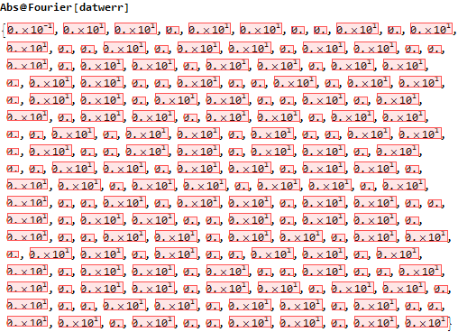


Fourierexample, it is working with machine numbers so no error tracking is happening and the ill conditioning matters. Compare to:In[1063]:= MinMax@ Map[Accuracy, Abs[Fourier[N[Table[Sin[2 \[Pi] t], {t, 0, 1, 1/50}], 100]]]] Out[1063]= {98.7152508426, 99.4973398215}I believe tnis also avoids error tracking by working with fixed precision (not absolutely certain however) but regardless the higher precision suffices to overcome the conditioning in this example. $\endgroup$NumericalMath`$NumberBits[0``10 + 10^-9]$\endgroup$