corrected wording about Fourier coefficient correlation
Source Link

dctData is the data you're asking about in your question, but I don't plot it directly here. In the 2nd graphic, where we show uncertainties from the inverse Fourier-transform, I think the uncertainties don't match the original because the 2nd bootstrap starts from the already Fourier-transformed data and assumes that the uncertainties in the coefficients are uncorrelated. However, we can show that the numbers Fourier coefficients are correlated with each other. You will need to take this into account if you do subsequent calculations with dctData. Lack of correlation tracking is also the reason why precision tracking can't be used for uncertainty analysis.

dctData is the data you're asking about in your question, but I don't plot it directly here. In the 2nd graphic, where we show uncertainties from the inverse Fourier-transform, I think the uncertainties don't match the original because the 2nd bootstrap starts from the already Fourier-transformed data and assumes that the uncertainties in the coefficients are uncorrelated. However, we can show that the numbers Fourier coefficients are correlated with each other. You will need to take this into account if you do subsequent calculations with dctData. Lack of correlation tracking is also the reason why precision tracking can't be used for uncertainty analysis.

dctData is the data you're asking about in your question, but I don't plot it directly here. In the 2nd graphic, where we show uncertainties from the inverse Fourier-transform, I think the uncertainties don't match the original because the 2nd bootstrap starts from the already Fourier-transformed data and assumes that the uncertainties in the coefficients are uncorrelated. However, we can show that the Fourier coefficients are correlated with each other. You will need to take this into account if you do subsequent calculations with dctData. Lack of correlation tracking is also the reason why precision tracking can't be used for uncertainty analysis.

Bounty Ended with 100 reputation awarded by rhermans
included some of my comments in the answer
Source Link
bootStrapUDList[listFuncHead_,data_]:=PlusMinus@@@MapThread[Through[{Mean,(Max@#-Min@#)/2&}@{##}]&,MapThread[listFuncHead[{##}]&,data/.pm_PlusMinus:>RandomVariate[UniformDistribution@Sort@{Subtract@@pm,Plus@@pm},200000]]]

bootStrapNDList[listFuncHead_,data_]:=PlusMinus@@@MapThread[Through[{Mean,StandardDeviation}@{##}]&,MapThread[listFuncHead[{##}]&,data/.pm_PlusMinus:>RandomVariate[NormalDistribution@@pm,200000]]]

Short[InputForm[data=Table[PlusMinus[Sin[2\[Pi] t]+RandomReal[{-10^-3,10^-3}],10^-3+10^-2t],{t,0,2,0.01}]],5]
(*{-0.00015902041160618116 ± 0.001, 0.06369389709857176 ± 0.0011, 0.12615800788307047 ± 0.0012000000000000001, 0.18766842577245152 ± 0.0013, 0.24919853862147867 ± 0.0014, <<193>>, -0.12457700878215405 ± <<1>>, -0.06205334281024041 ± 0.020900000000000002, 0.0009467025819242354 ± 0.021}*)

(*dctData is the data you're asking about in your question, but I don't plot it directly
here*)
Short[InputForm[dctData=bootStrapNDList[FourierDCT,data]],5]
(*{-0.00013058978084242337 ± 0.01243461722327339, 2.3922514484284694 ± 0.009345519847128744, 0.0004364938928370489 ± 0.008935073841291516, 5.06557192629556 ± 0.008842253876933912, <<195>>, 0.0003672953018113705 ± 0.008634731807823369, 0.0007823963956902927 ± 0.008202728384246478}*)

Short[InputForm[invDCTData=bootStrapNDList[FourierDCT[#,3]&,dctData]],5]
(*{-0.0001489981017240066 ± 0.012484433568524647, 0.06363813654805517 ± 0.012452403598913883, 0.1261974349932789 ± 0.012437140396949981, 0.18770987190793406 ± 0.012447580994827578, <<195>>, -0.062018564059908 ± 0.012431168492616582, 0.0010387203700553621 ± 0.012455374980166786}*)

ListPlot[#,PlotMarkers->Automatic]&/@Outer[#1/@#2&,{First,Last},{data,invDCTData},1]

dctData is the data you're asking about in your question, but I don't plot it directly here. In the 2nd graphic, where we show uncertainties from the inverse Fourier-transform, I think the uncertainties don't match the original because the 2nd bootstrap starts from the already Fourier-transformed data and assumes that the uncertainties in the coefficients are uncorrelated. However, we can show that the numbers Fourier coefficients are correlated with each other:. You will need to take this into account if you do subsequent calculations with dctData. Lack of correlation tracking is also the reason why precision tracking can't be used for uncertainty analysis.

Correlation[MapThread[FourierDCT[{##}]&,data/.pm_PlusMinus:>RandomVariate[NormalDistribution@@pm,20000]]];
Length@Cases[%,x_?NumericQ/;Abs@x>.25,Infinity]
MatrixPlot@%%
 
(*601*)
bootStrapUDList[listFuncHead_,data_]:=PlusMinus@@@MapThread[Through[{Mean,(Max@#-Min@#)/2&}@{##}]&,MapThread[listFuncHead[{##}]&,data/.pm_PlusMinus:>RandomVariate[UniformDistribution@Sort@{Subtract@@pm,Plus@@pm},200000]]]

bootStrapNDList[listFuncHead_,data_]:=PlusMinus@@@MapThread[Through[{Mean,StandardDeviation}@{##}]&,MapThread[listFuncHead[{##}]&,data/.pm_PlusMinus:>RandomVariate[NormalDistribution@@pm,200000]]]

Short[InputForm[data=Table[PlusMinus[Sin[2\[Pi] t]+RandomReal[{-10^-3,10^-3}],10^-3+10^-2t],{t,0,2,0.01}]],5]
(*{-0.00015902041160618116 ± 0.001, 0.06369389709857176 ± 0.0011, 0.12615800788307047 ± 0.0012000000000000001, 0.18766842577245152 ± 0.0013, 0.24919853862147867 ± 0.0014, <<193>>, -0.12457700878215405 ± <<1>>, -0.06205334281024041 ± 0.020900000000000002, 0.0009467025819242354 ± 0.021}*)

Short[InputForm[dctData=bootStrapNDList[FourierDCT,data]],5]
(*{-0.00013058978084242337 ± 0.01243461722327339, 2.3922514484284694 ± 0.009345519847128744, 0.0004364938928370489 ± 0.008935073841291516, 5.06557192629556 ± 0.008842253876933912, <<195>>, 0.0003672953018113705 ± 0.008634731807823369, 0.0007823963956902927 ± 0.008202728384246478}*)

Short[InputForm[invDCTData=bootStrapNDList[FourierDCT[#,3]&,dctData]],5]
(*{-0.0001489981017240066 ± 0.012484433568524647, 0.06363813654805517 ± 0.012452403598913883, 0.1261974349932789 ± 0.012437140396949981, 0.18770987190793406 ± 0.012447580994827578, <<195>>, -0.062018564059908 ± 0.012431168492616582, 0.0010387203700553621 ± 0.012455374980166786}*)

ListPlot[#,PlotMarkers->Automatic]&/@Outer[#1/@#2&,{First,Last},{data,invDCTData},1]

In the 2nd graphic, where we show uncertainties from the inverse Fourier-transform, I think the uncertainties don't match the original because the bootstrap starts from the already Fourier-transformed data and assumes that the uncertainties in the coefficients are uncorrelated. However, we can show that the numbers Fourier coefficients are correlated with each other:

Correlation[MapThread[FourierDCT[{##}]&,data/.pm_PlusMinus:>RandomVariate[NormalDistribution@@pm,20000]]];
Length@Cases[%,x_?NumericQ/;Abs@x>.25,Infinity]
MatrixPlot@%%
 
(*601*)
bootStrapUDList[listFuncHead_,data_]:=PlusMinus@@@MapThread[Through[{Mean,(Max@#-Min@#)/2&}@{##}]&,MapThread[listFuncHead[{##}]&,data/.pm_PlusMinus:>RandomVariate[UniformDistribution@Sort@{Subtract@@pm,Plus@@pm},200000]]]

bootStrapNDList[listFuncHead_,data_]:=PlusMinus@@@MapThread[Through[{Mean,StandardDeviation}@{##}]&,MapThread[listFuncHead[{##}]&,data/.pm_PlusMinus:>RandomVariate[NormalDistribution@@pm,200000]]]

Short[InputForm[data=Table[PlusMinus[Sin[2\[Pi] t]+RandomReal[{-10^-3,10^-3}],10^-3+10^-2t],{t,0,2,0.01}]],5]
(*{-0.00015902041160618116 ± 0.001, 0.06369389709857176 ± 0.0011, 0.12615800788307047 ± 0.0012000000000000001, 0.18766842577245152 ± 0.0013, 0.24919853862147867 ± 0.0014, <<193>>, -0.12457700878215405 ± <<1>>, -0.06205334281024041 ± 0.020900000000000002, 0.0009467025819242354 ± 0.021}*)

(*dctData is the data you're asking about in your question, but I don't plot it directly
here*)
Short[InputForm[dctData=bootStrapNDList[FourierDCT,data]],5]
(*{-0.00013058978084242337 ± 0.01243461722327339, 2.3922514484284694 ± 0.009345519847128744, 0.0004364938928370489 ± 0.008935073841291516, 5.06557192629556 ± 0.008842253876933912, <<195>>, 0.0003672953018113705 ± 0.008634731807823369, 0.0007823963956902927 ± 0.008202728384246478}*)

Short[InputForm[invDCTData=bootStrapNDList[FourierDCT[#,3]&,dctData]],5]
(*{-0.0001489981017240066 ± 0.012484433568524647, 0.06363813654805517 ± 0.012452403598913883, 0.1261974349932789 ± 0.012437140396949981, 0.18770987190793406 ± 0.012447580994827578, <<195>>, -0.062018564059908 ± 0.012431168492616582, 0.0010387203700553621 ± 0.012455374980166786}*)

ListPlot[#,PlotMarkers->Automatic]&/@Outer[#1/@#2&,{First,Last},{data,invDCTData},1]

dctData is the data you're asking about in your question, but I don't plot it directly here. In the 2nd graphic, where we show uncertainties from the inverse Fourier-transform, I think the uncertainties don't match the original because the 2nd bootstrap starts from the already Fourier-transformed data and assumes that the uncertainties in the coefficients are uncorrelated. However, we can show that the numbers Fourier coefficients are correlated with each other. You will need to take this into account if you do subsequent calculations with dctData. Lack of correlation tracking is also the reason why precision tracking can't be used for uncertainty analysis.

Correlation[MapThread[FourierDCT[{##}]&,data/.pm_PlusMinus:>RandomVariate[NormalDistribution@@pm,20000]]];
Length@Cases[%,x_?NumericQ/;Abs@x>.25,Infinity]
MatrixPlot@%%
(*601*)
explained why uncertainties aren't on top of each other
Source Link

I'm not yet sure what the implication ofIn the 2nd graphic is. I do know it is different when, where we show uncertainties from the inverse Fourier-transform, I switchthink the uncertainties don't match the original because the bootstrap starts from the already Fourier-transformed data and assumes that the uncertainties in the coefficients are uncorrelated. However, we can show that the numbers Fourier coefficients are correlated with each other:

Correlation[MapThread[FourierDCT[{##}]&,data/.pm_PlusMinus:>RandomVariate[NormalDistribution@@pm,20000]]];
Length@Cases[%,x_?NumericQ/;Abs@x>.25,Infinity]
MatrixPlot@%%

(*601*)
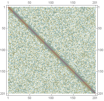
correlation coefficients matrix plot

In order to uniform distributions (UD version)show the uncertanties on top of each other, you would have to issue:

invDCTData=bootStrapNDList[FourierDCT[FourierDCT@#,3]&,data]]

But that would be rather boring.

I'm not yet sure what the implication of the 2nd graphic is. I do know it is different when I switch to uniform distributions (UD version).

In the 2nd graphic, where we show uncertainties from the inverse Fourier-transform, I think the uncertainties don't match the original because the bootstrap starts from the already Fourier-transformed data and assumes that the uncertainties in the coefficients are uncorrelated. However, we can show that the numbers Fourier coefficients are correlated with each other:

Correlation[MapThread[FourierDCT[{##}]&,data/.pm_PlusMinus:>RandomVariate[NormalDistribution@@pm,20000]]];
Length@Cases[%,x_?NumericQ/;Abs@x>.25,Infinity]
MatrixPlot@%%

(*601*)

correlation coefficients matrix plot

In order to show the uncertanties on top of each other, you would have to issue:

invDCTData=bootStrapNDList[FourierDCT[FourierDCT@#,3]&,data]]

But that would be rather boring.

add bootstrapping approach
Source Link
Loading
Source Link
Loading