Integrating an empirical probability density function

Question

I have created an empirical distribution that given an array containing the points px (e.g.{px0,px1,px2,px100}) the correspondent probability is given by a liner interpolation of the tipe:

The probability density function (PDF) corresponds to the angular coefficient m of the lines, which is computed in the function below.

GeneralEmpiricalDistribution[xdata_, pt_] := 
 Block[{n, tab, cdf, pdf, sz, i, index, m, x, x0, y0, xf, yf},
  sz = Length[xdata];
  n = sz - 2;
  tab = Table[{xdata[[i]], (i - 1)/(n + 1)}, {i, 1, n + 2}];
  For[i = 1, i < sz, i++,
   If[Between[pt, {xdata[[i]], xdata[[i + 1]]}], index = i; Break[] ];
   If[i == sz - 1, index = sz - 1]
   ];
  {x0, y0} = tab[[index]];
  {xf, yf} = tab[[index + 1]];
  m = (yf - y0)/(xf - x0);
  cdf = m (x - x0) + y0;
  pdf = m;
  {cdf, pdf}
  ]

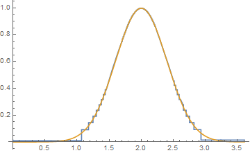
Then to validate the function above, consider the data (xdata) generated from a normal distribution with mean=2, and sdev=0.4:

mean = 2;
sdev = 0.4;
xdata = Table[Quiet[NSolve[CDF[NormalDistribution[mean, sdev], x] == prob, x][[1,1,2]]], {prob, 0.00000029, 1., 0.00999971}];
n = Length[xdata];
xmax = xdata[[n]];
Plot[{GeneralEmpiricalDistribution[xdata, x][[2]], 
PDF[NormalDistribution[mean, sdev], x]}, {x, 0, xmax}]

Which seems to be OK. But when i try to integrate to find the mean again the solution are very different:

NIntegrate[x GeneralEmpiricalDistribution[xdata, x][[2]], {x, 0, xmax}]
NIntegrate[x PDF[NormalDistribution[mean, sdev], x], {x, 0, xmax}]

Results:

0.0959046

1.99989

Why the integration results are different?

Answer 1

I mentioned this in a comment, but NIntegrate is evaluating the first argument, presumably so it can try to speed up the integration. Here's a way around that:

GeneralEmpiricalDistributionPDF[xdata_, pt_?NumericQ] :=
 GeneralEmpiricalDistribution[xdata, pt][[2]]

NIntegrate[x GeneralEmpiricalDistributionPDF[xdata, x], {x, 0, xmax}]
NIntegrate[x PDF[NormalDistribution[mean, sdev], x], {x, 0, xmax}]

NIntegrate::slwcon: Numerical integration converging too slowly; suspect one of the following: singularity, value of the integration is 0, highly oscillatory integrand, or WorkingPrecision too small.

NIntegrate::ncvb: NIntegrate failed to converge to prescribed accuracy after 9 recursive bisections in x near {x} = {2.93247}. NIntegrate obtained 1.9980823464466289` and 0.0025316961179251796` for the integral and error estimates.

1.99808

1.99989

Note that it complains about the function converging too slowly (might be because it's step-wise?). But the result is pretty much right.

---

Speeding up with Interpolation

By the way, here's a way to make the integration much faster and also more precise:

interpolatingGED[xdata_] :=

 With[{range = Range @@ Append[.1]@MinMax@xdata},
  Interpolation@
   Table[{x, GeneralEmpiricalDistribution[xdata, x][[2]]}, {x, 
     range}]
  ]

igedPDF[ig_, x_?NumericQ] :=
 ig[x]

With[{ig = interpolatingGED[xdata]},
 NIntegrate[x igedPDF[ig, x], {x, 0, xmax}] // RepeatedTiming
 ]

{0.016, 1.99893}

Basically we use an InterpolatingFunction to avoid the piece-wise discontinuous issue J.M. points out.

---

Speeding up with Compile

We can also write a compiled version of this which will be faster than the original.

gedParameters =
  Compile[{
    {xdata, _Real, 1},
    {pt, _Real}
    },
   Block[{n, tab, sz, i, index = -1, m, x0, y0, xf, yf},
    sz = Length[xdata]; n = sz - 2;
    tab = Table[{xdata[[i]], (i - 1)/(n + 1)}, {i, 1, n + 2}];
    Do[
     If[xdata[[i]] <= pt <= xdata[[i + 1]],
      index = i; Break[],
      If[i == sz - 1, index = sz - 1]
      ],
     {i, sz - 1}
     ];
    {x0, y0} = tab[[index]];
    {xf, yf} = tab[[index + 1]];
    m = (yf - y0)/(xf - x0);
    {x0, y0, m}
    ],
    "RuntimeOptions" -> {"EvaluateSymbolically" -> False}
   ];

gedParameters[xdata, 
   RandomReal[{0.0008958563278208521`, 3.6092680307500435`}]] // 
  RepeatedTiming // First

0.000028

GeneralEmpiricalDistribution[xdata, 
   RandomReal[{0.0008958563278208521`, 3.6092680307500435`}]] // 
  RepeatedTiming // First

0.00042

This then speeds up the integration a lot:

Quiet@
  NIntegrate[
   x GeneralEmpiricalDistributionPDF[xdata, x], {x, 0, 
    xmax}] // RepeatedTiming
Quiet@
  NIntegrate[
   x gedParameters[xdata, x][[3]], {x, 0, xmax}] // RepeatedTiming

{0.910, 1.99808}

{0.054, 1.99808}

Answer 2

Since your CDF is piecewise linear, it makes sense to use Interpolation[] on it, with the setting InterpolationOrder -> 1:

xdat = Table[InverseCDF[NormalDistribution[2, 0.4], prob],
             {prob, 0.00000029, 1., 0.00999971}];

cdfEmpirical = Interpolation[MapIndexed[Prepend[(#2 - 1)/(Length[xdat] - 1), #1] &, xdat], 
                             InterpolationOrder -> 1, 
                             "ExtrapolationHandler" -> {Automatic,
                                                        "WarningMessage" -> False}]

where we use the undocumented "ExtrapolationHandler" setting to allow the function to extrapolate without throwing a warning. With this, the PDF is just cdfEmpirical'[x], which we can now use with NIntegrate[]

NIntegrate[x cdfEmpirical'[x], {x, 0, xdat[[-1]]}, 
           Method -> "InterpolationPointsSubdivision"]
   1.99802

where the preprocessor method "InterpolationPointsSubdivision" allows NIntegrate[] to split the function internally into sections NIntegrate[] can easily handle.