Draw from continuous-discrete distribution

Question

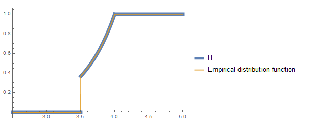
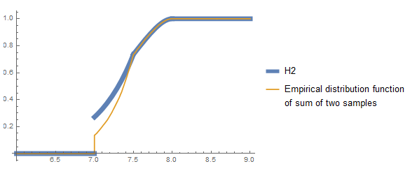
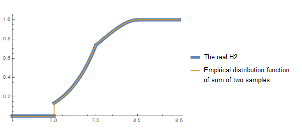
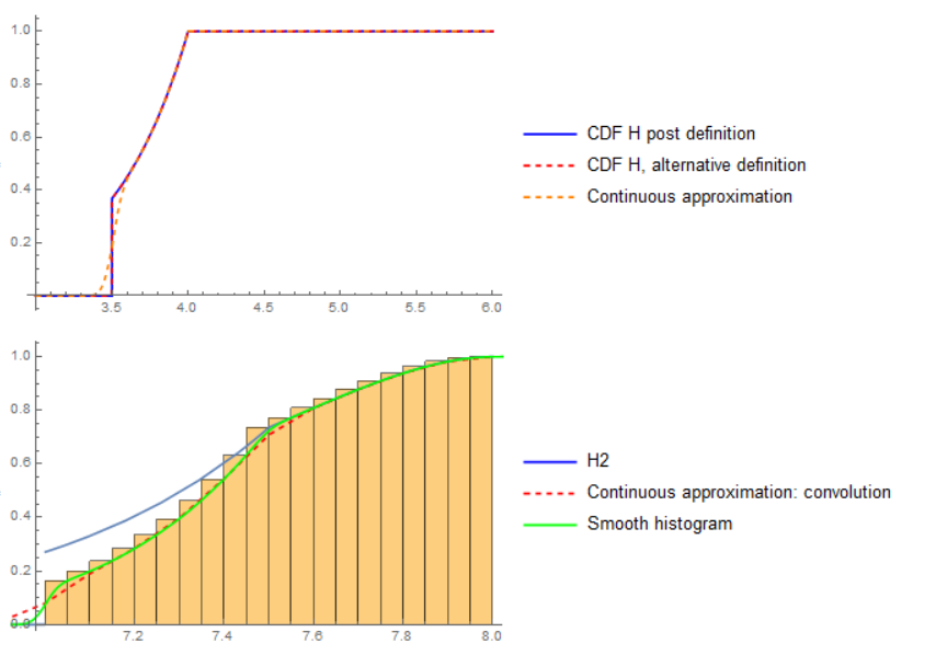
I have a random variable with a CDF that is almost everywhere differentiable, but has a point mass somewhere:

H21[s_] := Exp[lambda*(s - 2*nBar)] * (1 + lambda*(nBar - nUnder))
H22[s_] := Exp[lambda * (s - 2*nBar)] * (1 - lambda*(s - 2*nBar))
H2[s_] := Piecewise[{{H21[s], 
    2*nUnder <= s < nUnder + nBar}, {H22[s], 
    nUnder + nBar <= s < 2*nBar}, {1, s >= 2 * nBar}}, 0]
nBar = 4;
nUnder = 3.5;
lambda = 2;
Plot[{H2[s]}, {s, nUnder, 2 * nBar + 1}]

H2 here is the CDF. I believe that this CDF is corresponding to drawing twice from

$$ H(s) = \begin{cases} 0 & \text{ if } s < n_0 \\ e^{\lambda (s - n_1)} & \text{ if } n_0 \leq s \leq n_1 \\ 1 & \text{ if } s > n_1 \end{cases}$$

(where $n_0$, $n_1$ is what I call nUnder, nBar in my code).

I would like to verify that I computed $H_2$ correctly. So I would like to draw often from $H_2$, and compare that empirical distribution against drawing independent pairs from $H$ and adding them up.

I tried to follow this answer, but failed miserably.

custom[a_] := 
 ProbabilityDistribution[{"CDF", H2[x]}, {x, 2*nUnder, 2*nBar}]
g[a_] = CDF[custom[10], x];
h = Table[{g[x], x}, {x, 0, 40}] // N // 
   Interpolation[#, InterpolationOrder -> 0] &;
Show[h /@ (RandomReal[{0, 1}, {100}]) // 
  Histogram[#, Automatic, "Probability"] &, 
 Plot[PDF[custom[10], x - 1/2], {x, 0, 20}]]

After defining custom to be the ProbabilityDistribution as in the linked answer, I thought I was good to go (I carry around the unused parameter a_, but that should do no harm).

However, I get Interpolation::inddp: The point 0. in dimension 1 is duplicated when assigning h. What did go wrong - and how should I proceed?

Answer 1

It would seem sufficient to achieve the objective by obtaining the empirical distribution of a large number of samples of the sum of two independent observations and compare it to H2 rather than an empirical distribution built from samples from H2.

First define H for a single sample:

nBar = 4;
nUnder = 7/2;
lambda = 2;

H[s_] := Piecewise[{{0, s < nUnder}, {Exp[lambda (s - nBar)], nUnder <= s <= nBar},
  {1, s > nBar}}, 0]

Create a function to draw multiple samples from H and compare the empirical distribution from a large number of samples to H:

rSample[nSamples_, lambda_, nUnder_, nBar_] :=
 If[# <= Exp[lambda (nUnder - nBar)], nUnder, (nBar*lambda + Log[#])/lambda] &
   /@ RandomReal[{0, 1}, nSamples]

ed = EmpiricalDistribution[rSample[10000, lambda, nUnder, nBar]];
Plot[{H[s], CDF[ed, s]}, {s, nUnder - 1, nBar + 1},
 PlotStyle -> {Thickness[0.02], Thickness[0.005]},
 PlotLegends -> {"H", "Empirical distribution function"}]

Visually things look just fine.

Now essentially do the same thing but with taking the sum of two samples and compare against H2:

H21[s_] := Exp[lambda*(s - 2*nBar)]*(1 + lambda*(nBar - nUnder))
H22[s_] := Exp[lambda*(s - 2*nBar)]*(1 - lambda*(s - 2*nBar))
H2[s_] := Piecewise[{{H21[s], 2*nUnder <= s < nUnder + nBar},
  {H22[s], nUnder + nBar <= s < 2*nBar}, {1, s >= 2*nBar}}, 0]


ed = EmpiricalDistribution[
   rSample[10000, lambda, nUnder, nBar] + 
   rSample[10000, lambda, nUnder, nBar]];
Plot[{H2[s], CDF[ed, s]}, {s, 2 nUnder - 1, 2 nBar + 1},
 PlotStyle -> {Thickness[0.02], Thickness[0.005]},
 PlotLegends -> {"H2", 
   "Empirical distribution function\nof sum of two samples"}]

If the above steps are correct, it would seem that the definition of H2 needs work.

Update: Here is the real H2 you want

rSample[nSamples_, lambda_, nUnder_, nBar_] :=
  If[# <= Exp[lambda (nUnder - nBar)], nUnder, (nBar*lambda + Log[#])/lambda] &
  /@ RandomReal[{0, 1}, nSamples]

H2[s_, lambda_, nUnder_, nBar_] := Piecewise[{{0, s < 2 nUnder},
 {E^((nUnder - nBar) 2 lambda), s == 2 nUnder},
 {E^((-2 nBar + s) lambda) (1 - 2 nUnder lambda + s lambda), 2 nUnder < s <= nUnder + nBar},
 {E^((-2 nBar + s) lambda) (1 + 2 nBar lambda - s lambda), nUnder + nBar < s <= 2 nBar}},
 1]

nBar = 4;
nUnder = 7/2;
lambda = 2;
ed = EmpiricalDistribution[
   rSample[10000, lambda, nUnder, nBar] + 
   rSample[10000, lambda, nUnder, nBar]];

Plot[{H2[s, lambda, nUnder, nBar], CDF[ed, s]}, {s, 2 nUnder - 0.5, 2 nBar + 0.5},
 PlotStyle -> {Thickness[0.02], Thickness[0.005]},
 PlotLegends -> {"The real H2", "Empirical distribution function\nof sum of two samples"}]

Answer 2

Just to show similar left tail issue:

In the following the definition of H2 in the original post is used. First an alternative way to define the mix continuous and discrete distribution is shown. This is sampled to provide estimate of distribution of sum of independent variables. Then a continuous approximation using a "spike" normal distribution.

td = TransformedDistribution[3.5 z, 
   z \[Distributed] BernoulliDistribution[1]];
pd[x_] := 
  Piecewise[{{0, x <= 3.5}, {Exp[2 (x - 4)], 3.5 < x <= 4}, {1, 
     x > 4}}];
pr = ProbabilityDistribution[{"PDF", 
    2 Exp[2 (x - 4)]/Integrate[2 Exp[2 (u - 4)], {u, 3.5, 4}]}, {x, 
    3.5, 4}];
md = MixtureDistribution[{Exp[-1], 1 - Exp[-1]}, {td, pr}];
p1 = Plot[{CDF[md, x], pd[x]}, {x, 3, 6}, 
   PlotStyle -> {Blue, {Red, Dashed}}, Exclusions -> None];
pl = Show[
   Histogram[rv = Plus @@@ RandomVariate[md, {1000000, 2}], Automatic,
     "CDF"], Plot[H2[x], {x, 4, 8}]];
mix = MixtureDistribution[{Exp[-1], 
    1 - Exp[-1]}, {NormalDistribution[3.5, 0.05], pr}];
Legended[Show[p1, 
  Plot[CDF[mix, x], {x, 3, 6}, 
   PlotStyle -> {Directive[Orange, Dashed]}]], 
 LineLegend[{Blue, {Red, Dashed}, {Orange, 
    Dashed}}, {"CDF H post definition", 
   "CDF H, alternative definition", "Continuous approximation"}]]
con[w_] := 
 NIntegrate[
  PDF[mix, z] PDF[mix, s - z], {z, -Infinity, 
   Infinity}, {s, -Infinity, w}]
Legended[Show[pl, 
  ListPlot[Table[{j, con[j]}, {j, 6, 8.0, .1}], Joined -> True, 
   PlotStyle -> Directive[Red, Dashed]], 
  SmoothHistogram[rv, Automatic, "CDF", PlotStyle -> Green]], 
 LineLegend[{Blue, {Red, Dashed}, Green}, {"H2", 
   "Continuous approximation: convolution", "Smooth histogram"}]]

Answer 3

For mixed continuous and discrete distribution, MixtureDistribution will not work, ProbabiltyDistribution with Piecewise CDF function will also not work. Using direct function expression with DiracDelta function instead. The following is an example of tested work way:

\[ScriptCapitalD]1=ProbabilityDistribution[(m n)/(m+n) x^(-1+m)+m/(m+n) DiracDelta[x-1],{x,0,1},Assumptions->m>0&&n>0]