NIntegrate not giving the correct value

Question

I have an integrand which cannot be integrated analytically:

pr[x_] = -Pi/4 x^2 Cos[x^2] FresnelC[Sqrt[2] x/Sqrt[Pi]]^2;

but I also have an approximation to it:

g[x_] = Sqrt[\[Pi]/2]/(16 x) - Cos[x^2]/32 + (3 Cos[x^2])/(128 x^4) - 
   1/16 \[Pi] x^2 Cos[x^2] + (Sqrt[\[Pi]/2] Cos[2 x^2])/(16 x) + 
   1/32 Cos[3 x^2] - (7 Cos[3 x^2])/(128 x^4) - (3 Sin[x^2])/(
   128 x^6) + Sin[x^2]/(32 x^2) + (3 Sqrt[\[Pi]/2] Sin[2 x^2])/(
   32 x^3) - 1/8 Sqrt[\[Pi]/2] x Sin[2 x^2] - (3 Sin[3 x^2])/(
   128 x^6) + Sin[3 x^2]/(32 x^2);

I try to estimate the error between the integrand and its approximation by doing:

NIntegrate[pr[x] - g[x], {x, 10, ∞}, 
  Method -> "MonteCarlo",
  PrecisionGoal -> 10]

but it gives me a large value (-7e8) whereas I know that it should be very small.

How do I correct the numerical integration?

Answer 1

The integrand, as an exact function, seems a reasonably well-behaved oscillatory function that can be integrated (numerically) successfully via extrapolation; however, as a numerical function, it is horrible. (Expect the code below to run slowly, from seconds to minutes.) To evaluate at x -> 100. accurately you need 4343 digits of accuracy, or you'll be way off:

pr[x] - g[x] /. {{x -> 100.`4342}, {x -> 100.`4343}};
% // N
Precision /@ %%
(*
  {0.00136186, -5.3138*10^-11}
  {26.7328, 4323.03}
*)

All I think of is that there is some internal catastrophic cancellation that goes undetected. Note also that because of the need

Another possible issue, dwarfed by the precision one, is that the linear system constructed by the Levin rule is of dimension 48. Mathematica balks at solving this system at high precision. Perhaps with a significantly higher "TimeConstraint", it might work.

The built-in "ExtrapolatingOscillatory" strategy seems a good candidate, but it turns out that it cannot parse the complicated integrand. However we can imitate, as was done in How to find a more precise value of integral?

Borrowing again from Anton Antonov's answer, we can divide the interval of integration up at x == Sqrt[2 Pi * i] and represent it as a sum integrals between the nodes. I put a Check[] on the integral so I could investigate ones that did not converge. We'll also be using the terms repeatedly, so it's good to memoize their values.

ClearAll[term];
mem : term[i_?NumberQ] := mem = Module[{iRes},
    Check[
     iRes = NIntegrate[(pr[x] - g[x]), {x, Sqrt[2 Pi*i], Sqrt[2 Pi*(i + 1)]},
       PrecisionGoal -> 20, AccuracyGoal -> 20, 
       WorkingPrecision -> 40 + 3 i, 
       Method -> {"GaussKronrodRule", "Points" -> 15}],
     Print["i = ", i]
     ];
    iRes];

To make it easy to code, I picked x == Sqrt[2 Pi*i], i = 16, 17, ... for the nodes, but it leaves a little bit of the OP's integral from x == 10 to x == Sqrt[2 Pi*16] to be added:

bit = NIntegrate[pr[x] - g[x], {x, 10, Sqrt[2 Pi*16]},
  PrecisionGoal -> 10, WorkingPrecision -> 200]    
sf[n_] := Total@Table[SetPrecision[term[i], 200], {i, 16, n}]

We can then use Anton's SearchSumValue[] function (see below) to approximate the integral.

res = SearchSumValue[
  sf,                        (* partial sum function *)
  12,                        (* desired accuracy: abs. error < ~10^-12 *)
  30,                        (* number of terms to add each step *)
  40,                        (* starting number of terms *)
  Richardson[#1, #2, 24] &]  (* extrapolation function *)
answer = res[[2]] + bit      (* add the little bit to get the complete integral *)
(*
-7.4084729050246807289001990592571553616689002705033883146404497941764\
1713462740784131023302538755726602927879849993920908117244826729334375\
32927540835628437772008149977875*10^-6
*)

So the integral is estimated to be

-7.40847290*^-6

with an absolute error estimated by SearchSumValue[] to be at most 2.*^-15.

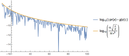
Further remarks (updated): The amplitude of pr[x] - g[x] appears to be about (15 Sqrt[(π/2)] )/(32 x^5), which can be seen from Simplify@Normal@Series[pr[x] - g[x], {x, Infinity, 5}]. I did a similar analysis as above with pr[x] - g[x] + (15 Sqrt[(π/2)] )/(64 x^5) with a different node grid and got the same result for the integral (subtracting the integral of (15 Sqrt[(π/2)] )/(64 x^5) from the sum, of course). Here is a comparison with the "amplitude" (15 Sqrt[(π/2)] )/(32 x^5) (takes a while to run):

Plot[{RealExponent[g[x] - pr[x]], RealExponent[(15 Sqrt[(π/2)] )/(32 x^5)]},
 {x, 10, 100}, MaxRecursion -> 2, PlotRange -> All, WorkingPrecision -> 5000,
 PlotLegends -> {HoldForm@Log10@Abs[pr[x] - g[x]], HoldForm@Log10[(15 Sqrt[(π/2)] )/(32 x^5)]}]

Code dump:

Clear[Richardson]
Richardson[A_, n_, N_] := 
 Total@Table[(A[n + k]*(n + k)^N*
      If[OddQ[k + N], -1, 1])/(k! (N - k)!), {k, 0, N}];

Clear[SearchSumValue]
SearchSumValue[partialSumFunc_, accGoal_, step_: 10, startStep_: 40, methodFunc_: Shanks] := 
  Block[{res, pf = 2}, 
   res = NestWhile[{#[[1]] + step, #[[3]], 
       methodFunc[partialSumFunc, #[[1]] + step]} &, {1, 
      methodFunc[partialSumFunc, startStep], 
      methodFunc[partialSumFunc, startStep + step]}, 
     Abs[N[#[[2]], pf*accGoal] - N[#[[3]], pf*accGoal]] > 10^-accGoal &];
   (*n-steps,estimate,error*)
   Append[res[[{1, 3}]], 
    Abs[N[res[[2]], pf*accGoal] - N[res[[3]], pf*accGoal]]]];