1
$\begingroup$

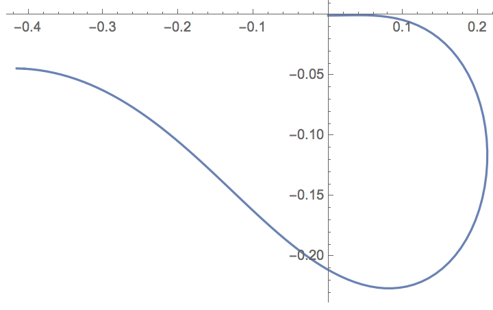
I need a parametric plot of a curve whose components are defined by:$$\left(\int_0^x\cos(f(t))dt,\int_0^x\sin(f(t))dt\right)$$ where $f(t)$ is an InterpolatingFunction (obtained from NDSolve). The Code I show below works fine, but depending on $f(t)$ can take very long to produce the output. Any suggestion to make it faster?...I mean, I am almost sure that the problem does not belong to ParametricPlot but to the way I define the integral with the variable extremum.

s = NDSolve[{y'[x] == g[x], g'[x] == -60 (1 - x) Cos[y[x]], y[0] == 0,g[0]== 1.2}, {y, g}, {x, 0, 1}];
f[x_] = Evaluate[y[x] /. s];
intcos[x_Real] := NIntegrate[Cos[f[t]], {t, 0, x}];
intsin[x_Real] := NIntegrate[Sin[f[t]], {t, 0, x}];
ParametricPlot[{intcos[x], intsin[x]}, {x, 0, 1}]

Note The code does not produce an output in mathematica 11, but work fine in mathematica 10, but I am going to make another question about that.

$\endgroup$
5
  • $\begingroup$ Where is f[t]? How can we test it? $\endgroup$
    – zhk
    Commented Apr 27, 2017 at 11:49
  • $\begingroup$ I added the information you need. Thanks! $\endgroup$
    – Popbatman
    Commented Apr 27, 2017 at 12:55
  • 3
    $\begingroup$ Possible duplicate of ParametricPlot does not work in Mathematica 11 as in 10 $\endgroup$
    – zhk
    Commented Apr 27, 2017 at 14:27
  • $\begingroup$ I was asking two different things about the same code. I think the best was to open two questions. $\endgroup$
    – Popbatman
    Commented Apr 27, 2017 at 14:29
  • $\begingroup$ Your both issues were answered by @Pillsy response, doesn't it? $\endgroup$
    – zhk
    Commented Apr 27, 2017 at 14:37

3 Answers 3

2
$\begingroup$

For this you already got an elegant answer from @Pillsy.

But here, I will propose an alternative approach using Table and Thread.

This is certainly faster than yours but not the one suggested by @Pillsy.

s = NDSolve[{y'[t] == g[t], g'[t] == -60 (1 - t) Cos[y[t]], y[0] == 0, g[0] == 1.2},
            {y, g}, {t, 0, 1}];

f[t_] = y[t] /. s[[1]];

intcos[x_Real] := NIntegrate[Cos[f[t]], {t, 0, x}];

intsin[x_Real] := NIntegrate[Sin[f[t]], {t, 0, x}];

incosdata = Table[intcos[x], {x, 0, 1, 0.02}];

insindata = Table[intsin[x], {x, 0, 1, 0.02}];

ListLinePlot[Thread[{incosdata, insindata}]]

enter image description here

$\endgroup$
0
$\begingroup$

It can be quicker if you use parallel computing.

In:

Clear[s, x, y, g, f, xys]
s = NDSolve[{y'[x] == g[x], g'[x] == -60 (1 - x) Cos[y[x]], y[0] == 0,
     g[0] == 1.2}, {y, g}, {x, 0, 1}];
f[x_] = Evaluate[y[x] /. s] // First ;
intcos[x_Real] := NIntegrate[Cos[f[t]], {t, 0, x}];
intsin[x_Real] := NIntegrate[Sin[f[t]], {t, 0, x}];
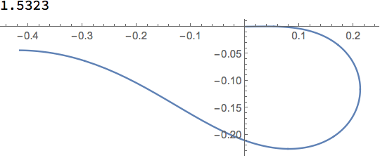
xys = ParallelTable[{intcos[x], intsin[x]}, {x, 0, 1, 
    0.01}]; (*Time is 2.84873 seconds, 4 Wolfram Kernels*)

ListLinePlot[xys]

Out: enter image description here

$\endgroup$
0
$\begingroup$
$Version

(*  "11.1.1 for Mac OS X x86 (64-bit) (April 18, 2017)"  *)

s = NDSolve[{y'[x] == g[x], g'[x] == -60 (1 - x) Cos[y[x]],
     y[0] == 0, g[0] == 1.2}, {y, g}, {x, 0, 1}][[1]];

Clear[f, intcos, intsin]

Note the use of NumericQ rather than Real.

Cases[{3.7, 2, Pi}, _Real]

(*  {3.7}  *)

Cases[{3.7, 2, Pi}, _?NumericQ]

(*  {3.7, 2, π}  *)


f[x_?NumericQ] := y[x] /. s

intcos[x_?NumericQ] :=
  NIntegrate[Cos[f[t]], {t, 0, x},
   Method -> {Automatic, "SymbolicProcessing" -> False}];
intsin[x_?NumericQ] :=
  NIntegrate[Sin[f[t]], {t, 0, x},
   Method -> {Automatic, "SymbolicProcessing" -> False}];

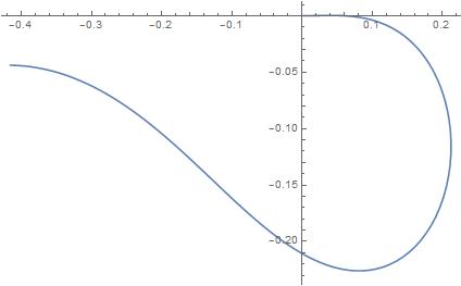
ParametricPlot[{intcos[x], intsin[x]}, {x, 0, 1},
   ImageSize -> Medium] // AbsoluteTiming // Column

enter image description here

$\endgroup$

Your Answer

By clicking “Post Your Answer”, you agree to our terms of service and acknowledge you have read our privacy policy.

Not the answer you're looking for? Browse other questions tagged or ask your own question.