How can I differentiate numerically?

Question

Mathematica has two ways to integrate: Integrate and NIntegrate.
But what about D? D and Derivative are for symbolic differentiation.

How can I differentiate a function numerically?

Answer 1

There are two rather different scenarios for numerical derivatives:

1. Differentiating a continuous function that's only defined numerically
2. Approximating the derivative of a list of data that could itself be generated numerically

For scenario 1, here is an example function and its derivative:

f[x_?NumericQ] := BesselJ[1, x]

Needs["NumericalCalculus`"]

Plot[ND[f[x], x, y], {y, 0, 10}]

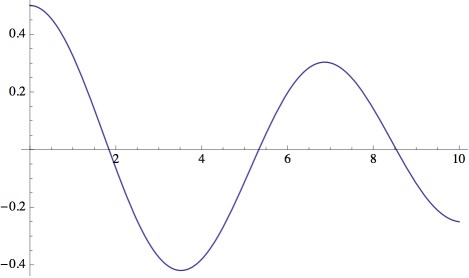
For scenario 2, here I discretize the above function to get a table of values in some interval:

l = Table[f[x], {x, 0, 10, .1}];

Now the derivative can be taken using DerivativeFilter. This doesn't require the "NumericalCalculus" package:

dl = With[{pad = 10},
   ArrayPad[
    DerivativeFilter[
     ArrayPad[l, pad, "Extrapolated"], {1}],
    -pad]
   ];

ListPlot[dl]

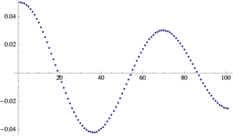
Here, I took the list l and padded it (optional) with pad extra entries at the start and end, before taking the numerical derivative using DerivativeFilter. The purpose of the padding is that it allows me to extrapolate the data points so that the derivative at the interval boundaries will look smooth.

After doing the derivative, I remove the padding by using a negative argument in ArrayPad[..., -pad].

Answer 2

As others mentioned, there's the ND function from the NumericalCalculus` package.

It's a bit less widely known that Derivative is also able to approximate derivatives purely numerically.

Let's create a numerical black box function:

f[x_?NumericQ] := x^2

_?NumericQ makes sure that the innards of f are inaccessible to Derivative, so f'[x] returns unevaluated. But plugging in an explicit numerical value,

In[]:= f'[3.]
Out[]= 6.

---

Update: Please also see a discussion by @acl concluding that the difference between Derivative and ND is that ND[...] takes the derivative from one side while N[D[...]] takes it symmetrically.

Answer 3

Had ND[] not been implemented in the NumericalCalculus` package, one could implement any number of numerical differentiation methods in Mathematica. I gave a number of warnings on the use of, as well as methods for, numerical differentiation in this MO answer; in particular, the last two methods I described lend themselves to somewhat compact implementations:

(* Cauchy method *)
ND1[f_, {x_, x0_}, opts___] :=
    Chop[NIntegrate[Exp[-I t] Function[x, f][x0 + Exp[I t]], {t, -Pi, Pi}, 
                    AccuracyGoal -> Infinity, opts, Method -> "DoubleExponential"]/(2 Pi)]

(* Lanczos method *)
ND2[f_, {x_, x0_}, opts___] := Module[{prec = Precision[x0], h, pr2}, 
    If[prec === Infinity, prec = MachinePrecision]; 
    h = # (Abs[x0] + #) &[(10^-(prec/2))];
    If[prec === MachinePrecision, pr2 = $MachinePrecision, pr2 = prec];
    N[3 NIntegrate[t Function[x, f][t + x0], {t, -h, h}, opts, 
                   WorkingPrecision -> pr2]/(2 h^3), prec]]

Both approaches are easily generalized; the Lanczos method can be generalized to arbitrary integer-order derivatives, and the Cauchy method can be generalized to arbitrary complex-order derivatives. I won't be discussing these generalizations further in this answer, tho.

A demonstration:

Plot[{-BesselJ[1, x], ND1[BesselJ[0, t], {t, x}]}, {x, 0, 10}, Axes -> None,
     Frame -> True, PlotStyle -> {Directive[Gray, Thick, Dashed], Blue}]

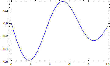
It's not too hard to implement the Richardsonian method I alluded to in my MO answer, but the routine is somewhat longer; I'll edit this answer to include it if there's interest.

Answer 4

I present here another approach to numerically differentiating a function $f(x)$. While the methods in my other answer approximate $f^\prime(x)$ at a single specified value, the following method constructs an approximate function $p(x)$ such that $p(x)\approx f(x)$ within a given interval $[a,b]$, and then proceeds to directly generate $p^\prime(x)$.

The key here is to replace the function with its Chebyshev series, and then differentiate that series. This is similar to what is done in the Chebfun package for MATLAB, and previously presented in a number of answers by Michael E2 and yours truly.

To recall, this is how one might derive the coefficients of the Chebyshev series of a function over a given interval (as previously shown here):

f[x_] := BesselJ[0, x];
{a, b} = {0, 19}; (* interval of approximation *)

n = 128; (* arbitrarily chosen integer *)
prec = 20; (* precision *)
cnodes = Rescale[N[Cos[π Range[0, n]/n], prec], {-1, 1}, {a, b}];
fc = f /@ cnodes;
cc = Sqrt[2/n] FourierDCT[fc, 1];
cc[[{1, -1}]] /= 2;

Then, one can either take the dot product of the Chebyshev coefficients cc with an appropriate list of suitably scaled Chebyshev polynomials (of the first kind), or use a more efficient evaluation method such as Clenshaw's algorithm, which was presented in these two answers. For simplicity, I will use the dot product method here:

Plot[{f[x], cc.ChebyshevT[Range[0, n], Rescale[x, {a, b}, {-1, 1}]]},
     {x, a, b}, PlotStyle -> {AbsoluteThickness[4], AbsoluteThickness[1]}]

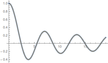
Now, one might be tempted to use D[] on the constructed Chebyshev series, but the problem with this approach is that ChebyshevT[] automatically converts to its power basis form for non-numeric arguments, thus negating any stability gained from remaining in the Chebyshev basis. Instead, one should directly construct the Chebyshev coefficients of the derivative.

The way to do that is to use a Chebyshev spectral differentiation matrix. What follows is a routine (previously posted here) to generate it.

chebmat[n_Integer?Positive, prec_: MachinePrecision] := 
 Module[{fac, xm},
        xm = ConstantArray[N[-Cos[π Range[0, n]/n], prec], n + 1];
        fac = Flatten[{2, PadRight[{}, n - 1, {-1, 1}], 2 - 4 Mod[n, 2]}];
        xm = Outer[Times, fac, 1/fac]/(xm - Transpose[xm] + IdentityMatrix[n + 1]);
        xm - DiagonalMatrix[Total[xm, {2}]]]

Now to generate the Chebyshev coefficients of the first derivative, do this:

dc = chebmat[n, prec].fc;
cd = FourierDCT[dc, 1] Sqrt[2/n] (2/(b - a));
cd[[{1, -1}]] /= 2;

Compare:

Plot[{f'[x], cd.ChebyshevT[Range[0, n], Rescale[x, {a, b}, {-1, 1}]]},
     {x, a, b}, PlotStyle -> {AbsoluteThickness[4], AbsoluteThickness[1]}]

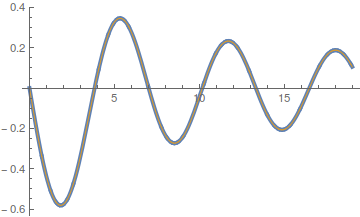
This approach is easily extensible to arbitrary order derivatives, just by multiplying fc with an appropriate power of chebmat[n]. For instance, here's how to generate the Chebyshev coefficients of the third derivative:

k = 3; (* derivative order *)
dck = MatrixPower[chebmat[n, prec], k, fc];
cdk = FourierDCT[dck, 1] Sqrt[2/n] (2/(b - a))^k;
cdk[[{1, -1}]] /= 2;

Answer 5

There is another possibility, and that is to differentiate an InterpolatingFunction.

Here is an example of a rather poorly behaving function whose derivative we can recover by this technique. The transfer function of a Butterworth filter looks like

h[s_] := 1 / (1 + 2s + 2s^2 + s^3)

for s complex. The Arg of this function, which, for purely imaginary frequencies, is the phase of the filter, suffers a branch cut at an inconvenient place:

Plot[Arg[h[I s]], {s, 0, 6}]

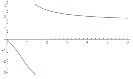
The symbolic derivative of this thing, which is group delay for the filter, bogusly produces Complex values, even if we didn't have the problem of the inconvenient branch cut:

Table[D[Arg[h[I s]], s] /. s -> t, {t, 0, 2}]

{ -2 I Arg', 
  (-(1/2) + 2 I) Arg'[-(1/2) - I/2], 
  (824/4225 - (118 I)/4225) Arg'[-(7/65) + (4 I)/65] }

We can get a better-behaved function by adding 2 Pi and then modding it out:

Plot[Mod[2 Pi + Arg[h[I s]], 2 Pi], {s, 0, 6}, PlotRange -> All]

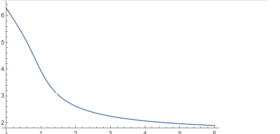
But now we have a "dimple" where we had the branch cut, and, sure enough, ND from NumericalCalculus has problems:

<< NumericalCalculus`
Plot[ND[Mod[2 Pi + Arg[h[I w]], 2 Pi], w, s], {s, 0, 6}, PlotRange -> Full]

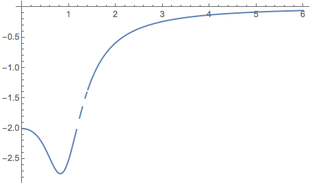
The DerivativeFilter method above works great to fix this, but here is another way. First, sample the original Arg or phase function:

ListPlot[args$ = Table[{s, Mod[2 Pi + Arg[h[I s]], 2 Pi]}, {s, .05, 6, .05}]]

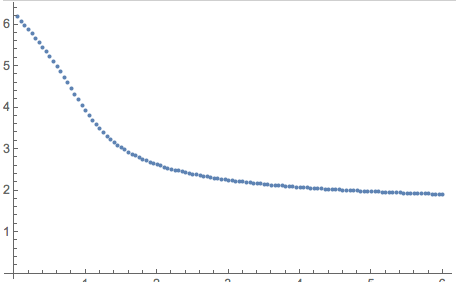
Build an interpolation function from it:

iargs$ = Interpolation[args$]

InterpolatingFunction[{{0.05, 6.}}, <>]

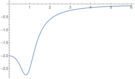
and differentiate that (notice carefully the tick mark in the following expression, a convenient shorthand for derivatives of functions of single variables):

Plot[iargs$'[s], {s, 0, 6}]