1
$\begingroup$

I am trying to integrate the following function,

f(r)=(80.50305990274495 - 35.03089630981622 r)/(80.50305990274495 - 
 79.5030598897815 r - r^2)
(* where r =[0,1] *)

The correct answer could be obtained by using NIntegrate command in Mathematica and it gave 13.027. The NIntegrate command always gave me 13.027 no matter what method I specify to integrate the integrand.

My main aim is to use Gauss Quadrature or other quadrature rules to get the correct result. Mathematica has a built-in command GaussianQuadratureWeights which generates the sampling points and the weights in an interval. Using following code I tried to integrate the function, f(r) using Gauss quadrature rule but i am not getting the correct result and the Reason is presence of singularity at one of the end points (r=1) due to which the convergence is very slow.

 nof=1500;
    f= (80.50305990274495` - 35.03089630981622` r)/(80.50305990274495` - 
 79.50305988978158` r - 1.` r^2) ;
    gq = GaussianQuadratureWeights[nof, 0, 1];
    xi = gq[[All, 1]];
    wi = gq[[All, 2]];
    sol = Sum[wi[[y]]*(f /. {r -> xi[[y]]}), {y, 1, nof}];

Ans: 9.24379 (which is not correct) Can anyone help me with this? Thanks ashu

$\endgroup$
5
  • $\begingroup$ How can I prove that ? Is there a way to calculate this using any other quadrature rules? $\endgroup$ Commented Jan 9, 2017 at 15:23
  • $\begingroup$ Your integrand has a value of 3.50774*10^9 at r -> 1, which contributes to the slow convergence of a straightforward rule application. NIntegrate overcomes this by subdividing the interval several times near r == 1.. You seem to appreciate this, but the implication is that the sampling has to be very high near r == 1. You might also need to increase the working precision to avoid roundoff error. $\endgroup$
    – Michael E2
    Commented Jan 9, 2017 at 16:27
  • $\begingroup$ Be aware the result is extremely sensitive to the difference between 80.50305990274495 and (1+79.50305988978158), which is ~10^-8. You are really pushing things trying to do this with machine precision. $\endgroup$
    – george2079
    Commented Jan 9, 2017 at 16:29
  • $\begingroup$ @MichaelE2 The slow convergence is due to singularity and NIntegrate is applying either some transformation or some other quadrature rule to avoid this singularity. I didn't specify the precision while using NIntegrate so I do not think that rounding off error would play major role. $\endgroup$ Commented Jan 9, 2017 at 16:43
  • $\begingroup$ (1) If you mean that the singularity is a little outside the interval, then, yes, that is what I was talking about. You have to expect slow convergence in that case. The further outside the singularity (relatively), the better the convergence, which is why in part recursive subdivision succeeds. (2) If you mean that the true singularity is at r == 1 (exactly) and not a little outside the interval, then you cannot assign a numeric value to the integral. It is a simple pole at the end point of the interval, and AFAIK, no regularization or principal value can be applied to yield a value. $\endgroup$
    – Michael E2
    Commented Jan 9, 2017 at 17:12

3 Answers 3

3
$\begingroup$

note this has an analytic solution:

res = Integrate[(a - b r)/(a - (a - 1 - eps)  r - r^2), {r, 0, 1}, 
  Assumptions -> {a > 0, b > 0, eps > 0}]

enter image description here

 res/.{a -> 80.50305990274495, 
       b -> 35.03089630981622, 
     eps -> 1.2963454310011002`*^-8}

13.027

Note the integrand is not singular, having a finite value (a-b)/eps (~10^9) at r=1, it is however not approximately polynomial which is I guess why Gauss integration doesn't work so well.

Edit:

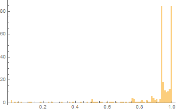
you may find this useful to see how NIntegrate does its adaptive sampling:

rules = {a -> 80.50305990274495, b -> 35.03089630981622, 
  eps -> 1.2963454310011002`*^-8}
xx = Reap[
    NIntegrate[
     Evaluate[(a - b r)/(a - (a - 1 - eps)  r - r^2) /. rules], {r, 0,
       1}, EvaluationMonitor :> Sow[r]]][[2, 1]];
Histogram[xx, {0, 1, .01}]

enter image description here

you see the vast majority of the sample points are taken near the (almost) singularity.

$\endgroup$
3
  • $\begingroup$ I appreciate your effort. But I want to get the same result using quadrature rules because I want a polynomial expression in terms of a, b and eps. May be using your methodology i could get something. Let me try. thanks $\endgroup$ Commented Jan 9, 2017 at 16:56
  • $\begingroup$ your quadrature scheme needs to sample points spaced on the order 10^-8 near r=1. Any more or less uniform sampling scheme (like Gauss) with then need on the order 10^8 sample points... (Not to mention I expect numerical precision errors if you try to go that route) $\endgroup$
    – george2079
    Commented Jan 9, 2017 at 17:11
  • $\begingroup$ Gauss quadrature works if I divide the interval into three sub-intervals (0 to 0.999, 0.999 to 0.99999 and 0.99999 to 1.0) I used 1000 nodes in each sub-interval except the first one where I used only 500 nodes. Is there a way to find out the number of nodes required for the convergence? $\endgroup$ Commented Jan 9, 2017 at 18:55
1
$\begingroup$

I don't know if this is an answer or a comment, but it shows how taming the singularity near r == 1 with a substitution makes the integration easier. The idea is that a substitution $r=g(u)$ transforms the integral of $f(r)$ into $$\int f(g(u))\,g'(u) \; du \,.$$ If $f(g(u))\,g'(u)$ remains bounded as $g(u)$ approaches the pole, then numerical integration should converge (as long as we stop short of the pole, as in the OP). This goal leads to a differential equation like $$f(g(u))\,g'(u)=1 \,,$$ which can be solved for the desired substitution $r=g(u)$. In the case of a pole at $r=b$, we can use $f(r)=1/(x-b)$ and solve $${1 \over g(u) - b}\,g'(u) = 1 \,.$$

wp = 35; (* working precision *)
Block[{$MinPrecision = wp, $MaxPrecision = wp, a, b},
 ff[r_] = SetPrecision[
   (80.50305990274495` - 35.03089630981622` r) / 
     (80.50305990274495` - 79.50305988978158` r - 1.` r^2),
   wp];
 gg[u_] = (* the substitution *)
  DSolveValue[{g'[u] == a (g[u] - b), g[0] == 0}, g[u], u] // Simplify;
 Off[Solve::ratnz];
 poles = Solve[1/ff[b] == 0];
 uend = u /.  (* end point of integration *)
   First[Solve[gg[u] == 1 /. a -> 1 /. Last[poles], u, Reals]];
 On[Solve::ratnz];
 
 nof = 15;
 gq = GaussianQuadratureWeights[nof, 0, uend, wp];
 xi = gq[[All, 1]];
 wi = gq[[All, 2]];
 a = 1;
 b = b /. Last[poles];  (* Last was determined by inspection *)
 sol = (ff@gg[xi] gg'[xi]).wi
 ]
% - NIntegrate[SetPrecision[ff[r], 2*wp], {r, 0, 1}, 
   WorkingPrecision -> 2*wp] // N
(*
  13.027018172900135745870557297655192
  -6.30971*10^-10  <-- error with 15 nodes
*)

One can increase the number of nodes up to 35-40 and the error will go down to 10^-26 or so, at which point the working precision needs to be increased to reduce the error.

$\endgroup$
0
$\begingroup$

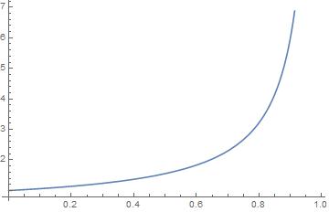
The function f goes to infinity when it gets close to r=1. So you will have some error integrating it numericaly.

f = (80.5031 - 35.0309 r)/(80.5031 - 79.5031 r - 1. r^2);
    Plot[f, {r, 0, 0.99}]
    Limit[f, r -> 1]
    NIntegrate[f, {r, 0, 0.99999999999947}]

enter image description here

What you can do to improve your solution is concetrate the fire int the most nonlinear region of the function. Here is the code:

<< NumericalDifferentialEquationAnalysis`
gq = GaussianQuadratureWeights[700, 0., 0.999999999];
xi1 = gq[[All, 1]];
wi1 = gq[[All, 2]];
gq = GaussianQuadratureWeights[700, 0.999999999, 1.];
xi2 = gq[[All, 1]];
wi2 = gq[[All, 2]];
Sum[wi1[[y]] (f /. {r -> xi1[[y]]}), {y, 1, Length[wi1]}] + 
 Sum[wi2[[y]] (f /. {r -> xi2[[y]]}), {y, 1, Length[wi2]}]
$\endgroup$
3
  • $\begingroup$ your code won't work here as at r=1 there is singularity. No matter how many gaussian nodes you consider in-between the interval 0.999999999 and 1, the results won't converge. The correct answer is 13.027. $\endgroup$ Commented Jan 9, 2017 at 15:56
  • $\begingroup$ Here NIntegrate[f, {r, 0,1.}] gives 54.774, and fails to converge. How do you know the rigth answer is 13.027? $\endgroup$
    – Stratus
    Commented Jan 9, 2017 at 16:06
  • $\begingroup$ check out the function f(r) again. It failed to converge because the earlier f(r) was not precise enough. Sorry for inconvenience. $\endgroup$ Commented Jan 9, 2017 at 16:09

Your Answer

By clicking “Post Your Answer”, you agree to our terms of service and acknowledge you have read our privacy policy.

Not the answer you're looking for? Browse other questions tagged or ask your own question.