6
$\begingroup$

Let's assume a vector of variables $\vec a=(a_1(t),a_2(t),a_3(t))$ and let's assume a following DE$$C\ddot{\vec a}=B\dot{\vec a}+A\vec{a}+\vec F.$$ If $A$ and $C$ are both reversible, than the DE can be written as $$\ddot{\vec a}=C^{-1}B\dot{\vec a}+C^{-1}A(\vec a+A^{-1}\vec F)$$ now making a crucial step $${(\vec a+A^{-1}\vec F)}''=C^{-1}B{(\vec a+A^{-1}\vec F)}'+C^{-1}A(\vec a+A^{-1}\vec F)$$ where $'$ still denotes a time derivative - it's just a cleaner syntax. By saying $(\vec a+A^{-1}\vec F)=\vec u$ we derived a very compact form of the second ordered DE system $${\vec u }''=C^{-1}B{\vec u}'+C^{-1}A\vec u.$$ To reduce the order from second to first we define yet another vector $\vec v={\vec u}'$. Doing so, our system can be rewritten in the following form $${\binom{\vec u}{\vec v}}'=\begin{pmatrix} 0 &I \\ C^{-1}A&C^{-1}B \end{pmatrix}\binom{\vec u}{\vec v}$$ which is in a $${\vec z}'=H\vec z$$ form and can be solved via eigensystems theories $$\vec z (t)=\sum C_k\vec \lambda _ke^{\lambda_kt}$$ for eigenvalues $\lambda_k$ and eigenvectors $\vec \lambda_k$.

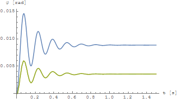
PROBLEM The system can be "easily" solved via NDSolve[]. The equations are

    equations = {800000. φ1[t] - 800000. φ3[t] + 
     0.105 (16858.8 Derivative[1][φ1][t] + 
        16858.8 Derivative[1][φ2][t] + 
        229 (-176.58 + 10.08 φ1''[t] + 
           6.93 φ2''[t] - 3.15 φ3'' [t])) == 0, 
   1.2*10^6 φ2[t] - 400000. φ3[t] + 
     0.105 (16858.8 Derivative[1][φ1][t] + 
        16858.8 Derivative[1][φ2][t] + 
        229 (-117.72 + 6.93 φ1''[t] + 
           6.3 φ2''[t] - 3.15 φ3''[t])) == 0, 
   1415.29 - 800000. φ1[t] - 400000. φ2[t] + 
     2.*10^6 φ3[t] - 75.7418 φ1''[t] - 
     75.7418 φ2''[t] + 60.5934 φ3''[t] == 0};

and using "brutal" NDSolve[]

n = 4;

variables = 
  Table[ToExpression["φ" <> ToString[i]], {i, 1, n}];


For[i = 1, i <= n - 1, i++, 
  AppendTo[equations, variables[[i]][t] == 0 /. t -> 0]];

For[i = 1, i <= n - 1, i++, 
  AppendTo[equations, D[variables[[i]][t], t] == 0 /. t -> 0]];

solution = 
  Quiet[NDSolve[Rationalize[equations], 
    Table[variables[[i]][t], {i, 1, n - 1, 1}], {t, 0, 5}]];

koti = Table[solution[[1, i, 2]], {i, 1, n - 1, 1}];

Plot[koti, {t, 0, 1.5}, PlotRange -> All, PlotLegends -> Automatic, 
 AxesLabel -> {"t [s]", "φ [rad]"}, 
 BaseStyle -> {FontFamily -> "Courier New", FontSize -> 10}]

produces

enter image description here

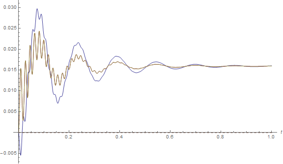
HOWEVER using all the theory written above and the code below produces something... well something that does not look the same. Make sure you clear the "equations" because at this point boundary conditions were added.

        matrixSecondD = 
  Normal@CoefficientArrays[
     equations, {φ1''[t], φ2''[t], φ3''[
       t]}][[2]];

matrixFirstD = -Normal@
    CoefficientArrays[
      Normal@CoefficientArrays[
         equations, {φ1''[t], φ2''[
           t], φ3''[t]}][[1]], {φ1'[
        t], φ2'[t], φ3'[t]}][[2]];

matrixZeroD = -Normal@
    CoefficientArrays[
      Normal@CoefficientArrays[
         Normal@
          CoefficientArrays[
            equations, {φ1''[t], φ2''[
              t], φ3''[t]}][[1]], {φ1'[
           t], φ2'[t], φ3'[t]}][[
        1]], {φ1[t], φ2[t], φ3[t]}][[2]];

matrixNonhomogeneousPart = -Normal@
    CoefficientArrays[
      Normal@CoefficientArrays[
         Normal@CoefficientArrays[
            equations, {φ1''[t], φ2''[
              t], φ3''[t]}][[1]], {φ1'[
           t], φ2'[t], φ3'[t]}][[
        1]], {φ1[t], φ2[t], φ3[t]}][[1]];

matrixSecondD.{φ1''[t], φ2''[t], φ3''[
     t]} == matrixFirstD.{φ1'[t], φ2'[
      t], φ3'[t]} + 
   matrixZeroD.{φ1[t], φ2[t], φ3[t]} + 
   matrixNonhomogeneousPart;

id = IdentityMatrix[3];

zeroes = ConstantArray[0, {3, 3}];

matrix = ArrayFlatten[{{zeroes, 
     id}, {Inverse[matrixSecondD].matrixZeroD, 
     Inverse[matrixSecondD].matrixFirstD}}];

eigenVal = Eigensystem[matrix][[1]];

eigenVec = Eigensystem[matrix][[2]];

constants = Table[ToExpression["C" <> ToString[i]], {i, 1, 2 (n - 1)}];

freeMatrix = Inverse[matrixZeroD].matrixNonhomogeneousPart;

equationSolution = 
  Sum[Table[
     constants[[i]]*Exp[eigenVal[[i]]*t] eigenVec[[i]] - 
      If[i <= (n - 1), freeMatrix[[i]], 0], {i, 1, Length[eigenVal], 
      1}][[j]], {j, 1, 2 (n - 1)}];

equationsForConst = 
  Table[equationSolution[[i]] == 0 /. t -> 0, {i, 1, 
    Length[eigenVal]}];

system = Solve[equationsForConst, constants];

constants = constants /. Flatten[system];

equationSolution = 
  equationSolution /. 
   Thread[Table[
      ToExpression["C" <> ToString[i]], {i, 1, 2 (n - 1)}] -> 
     constants];

koti = Drop[equationSolution, -(n - 1)];

Plot[Evaluate[ReIm /@ koti], {t, 0, 1}, PlotRange -> Full, 
 AxesLabel -> {t, None}, 
 PlotStyle -> (Sequence @@ {Directive[Thin, ColorData[1][#]], 
       Directive[Dashed, ColorData[1][#]]} & /@ Range[Length@koti]), 
 PlotLegends -> 
  Column@{LineLegend@*Sequence @@ 
     Transpose[{ColorData[1][#], "Eq. " <> ToString@#} & /@ 
       Range[Length@koti]], 
    LineLegend[{Thin, Dashed}, {"Real", "Imaginary"}]}, 
 ImageSize -> Large]

enter image description here

Why are solutions to the DE system not the same in both cases? And which one is the correct one? NOTE that this is the first time I am working with matrices in mathematica, so there is probably a really stupid mistake somewhere.

ps: that last part (plotting the real and imaginary party) is a copy paste code from Edmund in THIS answer.

$\endgroup$
23
  • 6
    $\begingroup$ Check you power cable for RF coupling :) $\endgroup$ Commented Mar 29, 2016 at 20:07
  • 1
    $\begingroup$ @Dr.belisarius: no comment :D made my day. $\endgroup$
    – skrat
    Commented Mar 29, 2016 at 20:18
  • $\begingroup$ Can you uses a simpler example for which you know the solution first? It's a bit early here, but how do you know that a = (a+A^(-1) F) Am I missing something? $\endgroup$
    – user21
    Commented Mar 29, 2016 at 21:17
  • $\begingroup$ You might want to correct your first code block so that it works properly; you seem to be taking derivatives using expressions like (φ1^′′)[t], which is definitely not right. $\endgroup$ Commented Mar 29, 2016 at 21:19
  • $\begingroup$ @user21: That's my defintion. Why do I use it? Because I couldn't find an easier way to convert my starting system into a final homogeneous system of first order DE - which I can solve via the eigensystem. Why u = (a+A^(-1) F) and not something else? Because with this definition I don't change the equation. Note that A^(-1) F is a constant vector. @MichaelSeifert: That's a notation this forum uses. If you copy paste the code in Mathematica, it should give you the derivatives. $\endgroup$
    – skrat
    Commented Mar 29, 2016 at 21:25

2 Answers 2

4
$\begingroup$

So Mathematica can, in fact, solve your equations exactly using DSolve instead of NDSolve:

solution = DSolve[equations, variables, t];
koti = {\[CurlyPhi]1[t], \[CurlyPhi]2[t], \[CurlyPhi]3[t]} /. solution;
Plot[Evaluate[Re /@ koti], {t, 0, 1}, PlotRange -> Full, 
           AxesLabel -> {t, None}, PlotPoints -> 100, ImageSize -> Large]

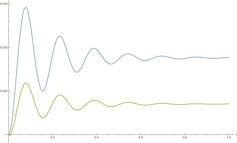
enter image description here

Note that I removed the Rationalize from equations before feeding it into DSolve. If you don't, Mathematica will try to work with exact roots of sixth-order polynomials, and that way lies madness.

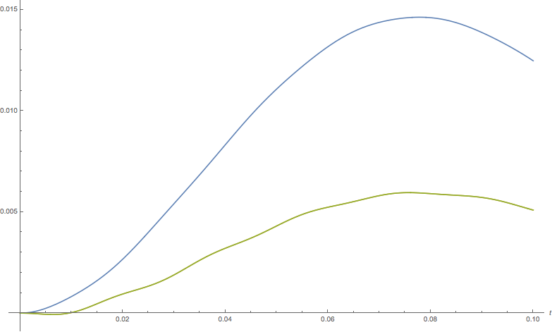
What I noticed in this graph is that the green graph is not as smooth as one would expect. This non-smoothness persists even if you increase the number of plot points (note the high value of PlotPoints in the above code) and if you zoom in on the graph:

enter image description here

This looks like a large oscillation with a very small oscillation superposed on it. Notably, in your second method, eigenVal works out to be

(* {-11.2869 + 344.474 I, -11.2869 - 344.474 I, -9.99201*10^-15 + 162.498 I, 
    -9.99201*10^-15 - 162.498 I, -5.40686 + 40.5931 I, -5.40686 - 40.5931 I} *)

and $2\pi/344.474 \approx 0.018$, which matches up nicely with the period of the small oscillations you can see on the graph above.

What I suspect is happening here is that your system has a high-frequency mode whose corresponding amplitude $C_k$ is low in the "true" solution. However, something is going wrong with your application of boundary conditions; resulting in this high-frequency oscillation being assigned a much higher amplitude $C_k$, making it noticeable.

In conclusion: the results of NDSolve and DSolve are generally consistent with each other. Moreover, a close examination of those two results has convinced me that there is an error in your home-brew method (in particular, the application of the initial conditions) that results in the weird-looking solution that is generated.

As an aside: DSolve is probably using a version of your algorithm to solve the equation exactly. But when I have a choice between using pre-tested algorithms to accomplish a task versus writing my own, I'll use the pre-tested algorithms every time.

$\endgroup$
3
  • $\begingroup$ My dear friend, I can't thank you enough! That's a very clear a nice explanation AND a super simple way to solve my system instead of what I was doing. Thank you big time: I had no idea Rationalize makes that much mess. Also thanks for making it clear what went wrong in my second method. $\endgroup$
    – skrat
    Commented Mar 30, 2016 at 22:13
  • $\begingroup$ However, after taking a closer look, does this explain the high difference in the stationary state? You can see for your self: My first plot (blue line) converges to some value below 0.010, yet the graph I got with the matrix method converges to a value above 0.015. That is... a lot relatively to the maximum value. $\endgroup$
    – skrat
    Commented Mar 31, 2016 at 13:44
  • $\begingroup$ @skrat. In case you missed the edit to my answer I got the matrix method to work (a1 converges to 0.00884556) $\endgroup$
    – george2079
    Commented Mar 31, 2016 at 15:35
4
$\begingroup$

It seems you have made some error, the eigensystem approach is shown to work:

First, You may find it useful to know that NDSolve can work directly with vector equations: (This is also validating the first part of your manipulation)

a={{8, 0, -8}, {0, 12, -4}, {-8, -4, 20}} 10^5
b={{1, 1, 0}, {1, 1, 0}, {0, 0, 0}} 1770.17
c={{-32, -22, 10}, {-22, -20, 10}, {10, 10, -8}} 7.57418
f={-3, -2, 1} 1415.29
ia = Inverse[a];
ic = Inverse[c];
sol = First@NDSolve[ {
          u''[t] == (ic.a).u[t] + (ic.b).u'[t] ,
            u[0] == ia.f,
           u'[0] == {0, 0, 0}
                               }, u[t], {t, 0, 5}]
aa[t_, i_] := (u[t] /. sol)[[i]] - (ia.f)[[i]]
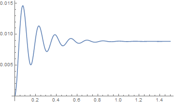
Plot[aa[t, 1], {t, 0, 1.5}, PlotRange -> All]

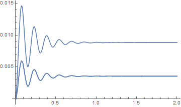
enter image description here

your first order form gives the same result:

h = {{ConstantArray[0, {3, 3}], IdentityMatrix[3]}, {ic.a, ic.b}};
sol = First@NDSolve[{
    {u'[t], v'[t]} == { 
      h[[1, 1]].u[t] + h[[1, 2]].v[t],
      h[[2, 1]].u[t] + h[[2, 2]].v[t]},
    {u[0], v[0]} == {ia.f, {0, 0, 0}}}, {u[t], v[t]}, {t, 0, 5}]

I think this capability is fairly new.. (this is v10.1). unfortunately it doesn't appear to generalize to higher order tensor this throws an error:

 NDSolve[{z'[t] == h.z[t], z[0] == {ia.f, {0, 0, 0}}}, z[t], {t, 0, 5}]

we can however pose this as a 6-vector, using a 6x6 form of h:

h66 = {
   Join[h[[1, 1, 1]], h[[1, 2, 1]]],
   Join[h[[1, 1, 2]], h[[1, 2, 2]]],
   Join[h[[1, 1, 3]], h[[1, 2, 3]]],
   Join[h[[2, 1, 1]], h[[2, 2, 1]]],
   Join[h[[2, 1, 2]], h[[2, 2, 2]]],
   Join[h[[2, 1, 3]], h[[2, 2, 3]]]};
(* surely some incantation of Flatten[h,levelspec] does the same..*)
sol = First@
  NDSolve[{z'[t] == h66.z[t], z[0] == Flatten[{ia.f, {0, 0, 0}}]}, 
   z[t], {t, 0, 5}]
aa[t_, i_] := (z[t] /. sol)[[i]] - (ia.f)[[i]]
Plot[aa[t, 1], {t, 0, 1.5}, PlotRange -> All]

same plot

Now we can apply your eigensystem solution:

{eval, evec} = Eigensystem[h66];
csol = First@
   Solve[ Sum[ cc[k] evec[[k]] , {k, 6}] == 
     Flatten[{ia.f, {0, 0, 0}}] , Array[cc, 6]];
eigsol = Sum[ (cc[k] /. csol) evec[[k]] Exp[eval[[k]] t], {k, 6}];
Plot[Table[Re[eigsol[[k]]] - (ia.f)[[k]], {k, 3}], {t, 0, 2}, 
   PlotRange -> All]

Exact same plot ( no noise ! )

enter image description here

limit value Chop[eigsol[[1]] - (ia.f)[[1]] /. t -> Infinity]

0.00884556

which is First@(-Inverse[a].f)

$\endgroup$
3
  • $\begingroup$ Thank you for your answer, maybe just one comment: Noise is not the problem - right the opposite: due to the physical laws of the system I would expect some superposition but absolutely not as much as I get with my matrix method described in the OP. $\endgroup$
    – skrat
    Commented Mar 31, 2016 at 16:56
  • $\begingroup$ i guess noise is not the right word. Your matrix solution shows a high frequency component not present in the direct solution. I'm guessing some error - compare your matrix with my h66 i think they should be the same although I didn't check that part of your code. $\endgroup$
    – george2079
    Commented Mar 31, 2016 at 17:36
  • $\begingroup$ This works nicely, but never came across that syntax koti[t_, i_] := (u[t] /. sol)[[i]] - (Inverse[matrixZeroD].matrixNonhomogeneousPart)[[i]] which works nicely for plotting but doesn't work at all if I want to use it in equation yKoordinateA = -l Sum[koti[t, i], {i, 1, n/2, 1}]; and plot yKoordinateA or get some numerical values. $\endgroup$
    – skrat
    Commented Mar 31, 2016 at 20:00

Your Answer

By clicking “Post Your Answer”, you agree to our terms of service and acknowledge you have read our privacy policy.

Not the answer you're looking for? Browse other questions tagged or ask your own question.