Radial distribution function

Question

I have tried to rewrite my old IDL code to calculate the radial correlation function for a regular 2D crystal structure.

The theory behind this function is given here: https://en.wikipedia.org/wiki/Radial_distribution_function

Update 1:

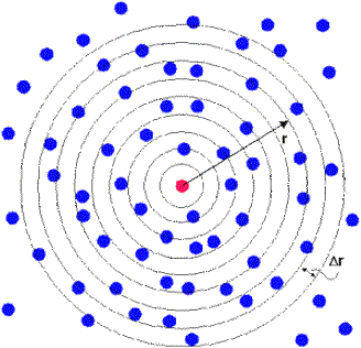
The radial density distribution counts the number of points in a distance between $r$ and $r +\Delta r$ from each considered central point (below one marked as red). The area of such a "shell" is $2\pi r \Delta r$. The density distributions are averaged for all center points and then normalized by the total point density times the ring area for each radius.

Update 2:

It is important that the maximum radius (the maximum shell) for each center point does not cross the edges of the available point coordiantes (corresponding to the range defined by the smallest and largest x and y point value). That means that a point close to the edges has a maller maximum radius (smallest distance to the next edge) than a center point (for a square: maximum radius = half of the diagonal).

My question: is it possible to improve my "unreadable" and slow code, which does not use any special mathematica functions?.

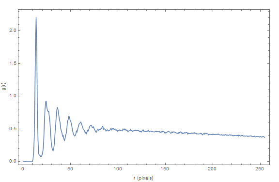
Also I must have made a normalization error, since the function does not converge at g(r)=1 (see plot below).

As input I have taken a crystal image recorded with a high resolution camera:

Dr. belisarius has detected all coordinates by the following one-liner:

pts = ComponentMeasurements[Binarize@ImageSubtract
   [image, BilateralFilter[image, 4, 1]], "Centroid"];

These points pts I have used to determine the radial correlation function.

The resulting plot is:

The full code is given here:

Clear[radialDensityDistribution];
radialDensityDistribution [listData_, mrr_: 0, mrc_: dDiag, 
  subdivision_: 50] :=
 (
  (*listData: list of 2D data points*)
  (*mrr: distance from edge*)
  (*mrc: calculation radius from central point*)
  (*subdivision: number of in size's from mean point distance*)

  n = Length[listData];

  x = listData[[All, 1]];
  y = listData[[All, 2]];

  minCorner = {Min[x], Min[y]};
  maxCorner = {Max[x], Max[y]};

  diag = maxCorner - minCorner;
  dDiag = Sqrt[diag.diag];

  area = diag[[1]]*diag[[2]];

  pointDensity = n/area;

  deltaR = (area/n)^(1.0/2);
  dr = deltaR/subdivision;

  maxShell = Floor[mrc/dr];

  g = Array[0 &, maxShell];
  centralPoint = Array[0 &, n];

  com = {Mean[x], Mean[y]};
  radii = Sqrt[(x - com[[1]])^2 + (y - com[[2]])^2];
  maxrad = Max[radii] // N;

  centralIndex = Flatten@Position[radii + mrr, n_ /; n <= maxrad];
  nCentral = Length[centralIndex];

  p = {x[[centralIndex]], y[[centralIndex]]};

  g = 0;

  Table[
   dist = {p[[1, 2 ;; All]] - p[[1, i]], 
      p[[2, 2 ;; All]] - p[[2, i]]}[[All, i ;; All]];
   shell = 
    Floor[Sqrt[
       dist[[1, All]]*dist[[1, All]] + dist[[2, All]]*dist[[2, All]]]/
      dr];
   h = HistogramList[shell, {0, maxShell - 1, 1}][[2, All]];
   g = h + g,
   {i, 1, nCentral - 1}
   ];

  Table[
   areaShell = Pi*(((shell + 1.0)*dr)^2 - (shell*dr)^2);
   g[[shell]] = g[[shell]]/(1.0*nCentral*areaShell*pointDensity),
   {shell, 1, maxShell - 1}
   ];

  rn = (Range[maxShell - 1] - 0.5)*dr;
  {g, rn, deltaR}
  )

image = Import["https://i.sstatic.net/czhuI.png"];

pts = ComponentMeasurements[
    Binarize@ImageSubtract[image, BilateralFilter[image, 4, 1]], 
    "Centroid"][[All, 2]];

extx = Max[pts[[All, 1]]] - Min[pts[[All, 1]]];
exty = Max[pts[[All, 2]]] - Min[pts[[All, 2]]];
ext = Min[extx, exty];

{g, rn, deltaR} = radialDensityDistribution [pts, ext/4, ext/4, 20];

ListLinePlot[Transpose[{rn, g}], PlotRange -> Full, Frame -> True, 
 FrameLabel -> {{"g(r)", ""}, {"r (pixels)", ""}}, ImageSize -> Large]

Answer 1

I will show a simple and fast approach to computing the pair correlation function (radial distribution function) for a 2D system of point particles.:

radialDistributionFunction2D[pts_?MatrixQ, boxLength_Real, nBins_: 350] :=
 Module[{gr, r, binWidth = boxLength/(2 nBins), npts = Length@pts, rho},
  rho = npts/boxLength^2; (* area number density *)
  {r, gr} = HistogramList[(*compute and bin the distances between points of interest*)
             Flatten @ DistanceMatrix @ pts, {0.005, boxLength/4., binWidth}];
  r = MovingMedian[r, 2]; (* take center of each bin as r *)
  gr = gr/(2 Pi r rho binWidth npts); (* normaliza g(r) *)
  Transpose[{r, gr}] (* combine r and g(r) *)
 ]

Here is how you use it:

rdf = radialDistributionFunction2D[pts, 1023.];
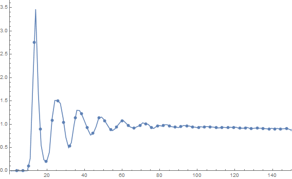
ListLinePlot[rdf, PlotRange ->{{0, 150}, All}, Mesh -> 80]

Notice that you get the correct normalization for free. This took about 1.2 seconds on my machine. I have restricted the plot range to show the interesting features.

Answer 2

"Disclaimer": This is solely an attempt to clean/speed up OP's code as it was presented, as I have not tried to figure out an alternative algorithm to do the calculation.

First a few comments:

• You might want to localize all the intermediate variables you use in a Block.
• When the deepest indice(s) in Part is All, we don't need to specify them. That is, p[[All,2,All,All]] is simply equivalent to p[[All,2]].
• Table is not a looping construct per se: Table produces a table of values, so unless we do something with the result (e.g. tab = Table[...]), we should use something else. In OP's case, they could be replaced with Do, but as we will see, we can do away with them entirely.

The bottleneck seems to be the calls to HistogramList, which happens nCentral times, 4397 in the example. There are two things we can do with this part of the code: turn the procedural g=0;Do[...;g=g+h] into a functional equivalent using Fold, and replacing HistogramList with a home-cooked, faster variant. We look at the last point first.

The bin specification {0, maxShell - 1, 1} gives unit bins $[0,1)$, $[1,2)$, etc., and since shell has integer values, HistogramList just tallies the values in shell that are less than maxShell - 1. Thus we can

1. Pick the shell values that are less than maxShell - 1
2. Tally a Sorted version of the result
3. Turn it into a SparseArray with default element 0 and correct length

Here is the code:

histList[shell_, maxShell_] :=
SparseArray[
  Rule @@ Transpose[Tally[1 +
    Sort[Pick[shell, Negative[shell - maxShell + 1]]]
  ]]
, maxShell - 1]

The g=0;Do[...;g=g+h] part can now be made functional using

gAcc[g_, i_] := Block[{dist, shell},
  dist = {p[[1, i + 1 ;; All]] - p[[1, i]], p[[2, i + 1 ;; All]] - p[[2, i]]};
  shell = Floor[Sqrt[dist[[1]]^2 + dist[[2]]^2]/dr];
  g + histList[shell, maxShell]
]

and finally

g = Fold[gAcc, 0, Range[nCentral - 1]];

On my machine this is about 4 times faster than OP's code.

Finally, the last part that modifies g can be vectorized, so no loop is necessary. Simply:

shells = Range[maxShell - 1];
areaShells = Pi*(((shells + 1.0)*dr)^2 - (shells*dr)^2);
g = g/(nCentral*areaShells*pointDensity);

Answer 3

image = Import@"https://i.sstatic.net/czhuI.png"; 
pts = ComponentMeasurements[Binarize@ImageSubtract[image, BilateralFilter[image, 4, 1]], 
                           "Centroid"][[All, 2]];

lpts = Length@pts;

(* the following is slow and not  really needed, we could take the center 
   to be at ImageDimensions/2 *)

nm = NMinimize[Tr[#.# & /@  Thread[Subtract[pts, {x0 + Cos[ArcTan[-y0 + #[[2]],
            -x0 + #[[1]]]], y0 + Sin[ArcTan[-y0 + #[[2]], -x0 + #[[1]]]]} & /@ 
                                     pts]]], {{x0, 400, 600}, {y0, 400, 600}}]

(*center*)
(*{9.29992*10^8, {x0 -> 504.879, y0 -> 505.181}}*)

ctr = {x0, y0} /. nm[[2]]
centeredPts = Subtract[#, ctr] & /@ pts;
xyLimits = Transpose[{-1/2 #, 1/2 #} &@ctr];
ptsInZone = Select[pts, xyLimits[[1, 1]] < #[[1]] < xyLimits[[1, 2]] &&
                        xyLimits[[2, 1]] < #[[2]] < xyLimits[[2, 2]] &];

f = Nearest[pts];

g[pt_, rad_] := Rest@f[pt, {lpts, rad}]
ran[n_] := Range[n, 250, n]
ptsAtAllRanges[pt_, n_] := g[pt, #] & /@ ran[n]

scale = 2;
pp = Differences[Length /@ ptsAtAllRanges[#, scale]] & /@ ptsInZone;
ListLinePlot[(Mean /@ Transpose@pp)/Rest@ran[scale], PlotRange -> All]

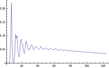
The horizontal scale is divided by 2: