RegionPlot: Incorrect Results

Question

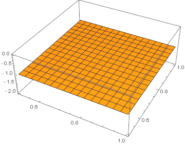
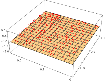
I have a simple function and I tried to simulate whether the resulting values are positive/negative/zero (all I want to know). I plotted the function with a set of parametric assumptions and the output made no intutive/mathematical sense (strange shapes with spikes). I picked a few coordinates, which are supposed to be nonnegative, and evaluated them individually. The results are contradictions.

Below are the two variables, the function, the assumptions, the RegionPlot for negative values only and three examples of contradictions. Unfortunately, the RegionPlot takes some time.

λupper1[α_, c_, e_, ϵ_, η_] := (-e + c η + α η)/(-c + α + c ϵ - α ϵ + c η + α η) // FullSimplify
λupper2[α_, c_, e_, ϵ_, η_, y_] := (c - y + (-e + y + α) η)/(-(e - y + α) (-1 + ϵ) + (-e + y + α) η) // FullSimplify
assumptions12 = α > 0 && e > 0 && c > 0 && α > e && α > c && y > c && y > e && y < e + c;
Simplify[Sign[λupper12[α, c, e, ϵ, η,  y] /. {ϵ -> 0.55, η -> 1}], assumptions12]
λupper12[α_, c_, e_, ϵ_, η_, y_] =λupper1[α, c, e, ϵ, η] -λupper2α, c, e, ϵ, η, y] // FullSimplify
RegionPlot[Simplify[λupper12[α, c, e, ϵ, η, y] < 0, assumptions12], {ϵ, 0.5, 1}, {η, 0.5, 1}]
Simplify[Sign[λupper12[α, c, e, ϵ, η, y] /. {ϵ -> 0.6, η -> 0.52}], assumptions12]
Simplify[Sign[λupper12[α, c, e, ϵ, η, y] /. {ϵ -> 0.85, η -> 0.8}], assumptions12]

Is there a way to get an accurate representation for lambdaupper12 in a diagram with epsilon and eta on the axes?

Thank you!

Answer 1

Below is a copy of your input (slightly modified). I wrote out the simplifications and removed α>0 as it was redundant.

λupper1[α_,c_,e_,ϵ_,η_] := (-e + (c + α) η)/(α (1 - ϵ + η) + c (-1 + ϵ + η))

λupper2[α_,c_,e_,ϵ_,η_,y_] := (c - y + (-e + y + α) η)/
   (-(e - y + α) (-1 + ϵ) + (-e + y + α) η)

λupper12[α_,c_,e_,ϵ_,η_,y_] = λupper1[α,c,e,ϵ,η] - λupper2[α,c,e,ϵ,η,y]

assumptions12 = e>0 && c>0 && α>e && α>c && y>c && y>e && y<e+c

Make a table

I attempted to make a table of the results and then use ListPlot3D. I discovered that some results were left in a symbolic state:

Simplify[Sign[λupper12[α, c, e, ϵ, η, y] /. {ϵ -> 0.5, η -> 0.61}], assumptions12]

The reason it is left in symbolic form is that when you substitue those particular values (0.5, 0.61) the expression inside the Sign becomes:

eq = (-e + 0.61 (c + α))/(
  0.11 c + 1.1 α) + (-c + 0.61 e + y - 
   0.61 (y + α))/(-0.5 (-e + y - α) + 
   0.61 (-e + y + α))

Now use Reduce to get a solution for the case where the expression is less than one and greater than one:

Reduce[(-e + 0.61 (c + α))/(
    0.11 c + 1.1 α) + (-c + 0.61 e + y - 
     0.61 (y + α))/(-0.5 (-e + y - α) + 
     0.61 (-e + y + α)) < 0 && e > 0 && 
  c > 0 && α > e && α > c && y > c && y > e && 
  y < e + c, {α, c, e, y}, Reals]

and

Reduce[(-e + 0.61 (c + α))/(
    0.11 c + 1.1 α) + (-c + 0.61 e + y - 
     0.61 (y + α))/(-0.5 (-e + y - α) + 
     0.61 (-e + y + α)) > 0 && e > 0 && 
  c > 0 && α > e && α > c && y > c && y > e && 
  y < e + c, {α, c, e, y}, Reals]

They both have solutions indicating that they depend on the other parameters.

All is not lost

Make the table of data. To simplify the work I will define a function.

f[ϵ_, η_] := Simplify[Sign[λupper12[α, c, e, ϵ, η, y]], assumptions12]

data = Table[{ϵ, μ, f[ϵ, μ]}, {ϵ, 0.5, 1, 0.01}, {μ, 0.5, 1, 0.01}]

This takes a long time. Most of the data is numeric but some is left in a symbolic state.

Purge the data of the symbolic elements.

positions = Position[data, {x_Real, y_Real, z_Integer}];

numericData = Extract[data, positions];

ListPlot3D[numericData]

The plot is somewhat uninteresting as everthing not symbolic is -1.

Let's identify the points where two solutions exist. We will assign a value of -0.9 to those points.

symbolicData = Cases[data, {x_?NumberQ, y_?NumberQ, z_Sign} ->
    {x, y, -0.9}, {2}];

Now plot those points on top of the surface that has valid solutions.

Show[
 ListPlot3D[numericData, PlotStyle -> {Opacity[0.5]}],
 Graphics3D[{
   Red,
   Point[symbolicData]
   }]
 ]