3
$\begingroup$

I'd like to compute the response of a TransferFunctionModel when driven by a SquareWave. Here's a simple example,

or = OutputResponse[TransferFunctionModel[1/(s + 1), s], SquareWave[t], t];

which results in two copies of the error:

Reduce::nsmet: This system cannot be solved with the methods available to Reduce. >>

Oddly, or still gets set to

{(-1 + Piecewise[{{-E^t, Inequality[1/2, LessEqual, Mod[t, 1], Less, 1]}}, E^t])/E^t}

which looks like this:
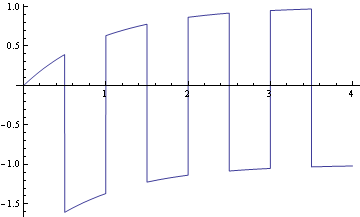
enter image description here

and is the correct response of the system to UnitStep[t], but multiplied by SquareWave[t].

How can OutputResponse be used to find the response of a TransferFunctionModel driven by a SquareWave?

$\endgroup$

3 Answers 3

1
$\begingroup$

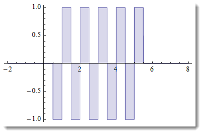
I think you are right about using finite sequence of pulses. But here is how you can get it still using SquareWave - you just need to introduce right cut-off. Then no sums over steps or pulses are needed and implementation is easy.

For example:

finiteSquareWave[t_] := UnitBox[.2 (t - 3)] SquareWave[t];
Plot[finiteSquareWave[t], {t, -2, 8}, Exclusions -> None,  Filling -> 0]

enter image description here

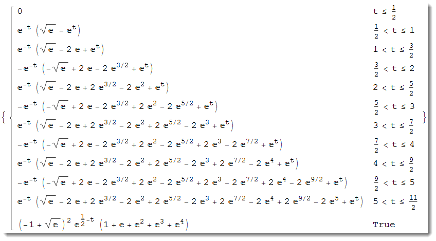
f[t_, z_] = OutputResponse[ TransferFunctionModel[1/(s + 1), s], finiteSquareWave[t], t]

enter image description here

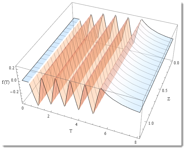
Plot3D[f[t, z], {z, 0, 1.2}, {t, 0, 8}, 
 AxesLabel -> {"Z", "T", "f(Z,T)"}, MeshFunctions -> {#1 &}, 
 PlotRange -> All, PlotStyle -> Opacity[.5], MeshStyle -> Opacity[.3]]

enter image description here

This is similar to what you got with sums over UnitSteps.

$\endgroup$
4
  • $\begingroup$ I like this one. When I attempt to change the phase of the SquareWave using finiteSquareWave[t_] := UnitBox[.2 (t - 3)] SquareWave[t - 0.1];, the error returns. Any idea why? $\endgroup$ Commented Aug 20, 2012 at 22:54
  • $\begingroup$ @ArgentoSapiens it is not an error, but just a message that solution is given not in an exact, but numerical form. Plotting function and other computations still work. $\endgroup$ Commented Aug 21, 2012 at 0:58
  • $\begingroup$ 3D plot looks pretty :-), but it's only a cylindrical function, so what's the third dimension for? $\endgroup$
    – stevenvh
    Commented Aug 21, 2012 at 8:37
  • $\begingroup$ @stevenvh f(z,t) - so 3 axis are z,t,f . It is a standard plot wolfram.com/xid/0g7kxbwzgfy-zycipu $\endgroup$ Commented Aug 21, 2012 at 8:56
4
$\begingroup$

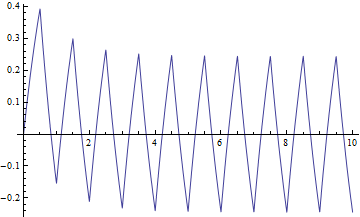
I hardly ever try to obtain an analytic expression from OutputResponse since I am really only interested in a plot of the response and an InterpolationFunction. So unless you have a need to see an analytical expression, use a numerical one. This happens when you provide a complete time specification as in {t,0,10} instead of just t.

Now you will obtain an InterpolationFunction which is for all practical purposes just as good. Not only is it faster, you know it will almost always work for any input.

In[3]:= or=OutputResponse[TransferFunctionModel[1/(s+1),s],SquareWave[t],{t,0,10}]    
Out[3]= {InterpolatingFunction[{{0.,10.}},<>][t]}

But if you insist you want an analytical response, then may be there is a way. But see first if the above works for you.

Plot[or, {t, 0, 10}]

enter image description here

$\endgroup$
1
$\begingroup$

A fake, finite-time version of SquareWave can be made thus:

sw = With[
 {period = 2},
 Sum[
  UnitStep[t - period/2 number] - UnitStep[t - period/2 (number + 1)],
  {number, 0, 10, 2}
 ]
]

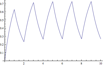
And this fake SquareWave works with OutputResponse:

or = OutputResponse[TransferFunctionModel[1/(s + 1), s], sw, t];
Plot[or, {t, 0, 10}]

enter image description here

$\endgroup$

Your Answer

By clicking “Post Your Answer”, you agree to our terms of service and acknowledge you have read our privacy policy.

Not the answer you're looking for? Browse other questions tagged or ask your own question.