When I first made this answer I was bleary eyed and didn't realize that Willinski's answer matched the question except that he made a nice edit by replacing, for example, 1.5 with 3/2.
This answer is in addition to Willinski's fine work. I followed his procedure.
I wanted to do a numerical study and try to find the region of interest.
A = 1;
J = 1;
c = 1;
beta = 1;

int = Integrate[E^(c*beta*l*H*(1.5 x^2 - 0.5)), {x, 0, 1}]//FullSimplify

sum1 = (1 + Sum[l^(3/2)*E^(-u*l)*int, {l, 1, 100}])
sum2 = (1 + Sum[l^(5/2)*E^(-u*l)*int, {l, 1, 100}])
Note that the integration in sum2 is identical to that used in sum1.
I defined a function representing equation 1, eq1 and equation 2, eq2.
eq1[u_, H_] = A*beta^(-3/2)*E^(-J*beta - 0.5*c*beta*H^2)*(sum1)

eq2[u_, H_] = A*beta^(-3/2)*E^(-J*beta - 0.5*c*beta*H^2)*(sum2)
Note: The function definitions don't use the normal SetDelay (:=) but rather use Set (=).
I first evaluted eq1 and eq2 over different ranges in order to get a birds eye view of where it fit the equation values of 1 and H.
I created data using Table and discriminated the results to lie within the answer for equation 1 (e.g., ≈ 1) and the answer for equation 2 (e.g., ≈ H).
eq1data is for equation 1 and eq2data is for equation 2.
eq1data = Table[{u, H, eq1[u, H]}, {u, 0.1, 2, 0.1}, {H, 0.1, 1, 0.1}];

eq1data =
  DeleteCases[
   Map[Function[subList, Select[subList, #[[3]] < 2. &]],
    eq1data], {}];

eq1data = Partition[Flatten[eq1data], 3];

eq2data = Table[{u, H, eq2[u, H]}, {u, 0.1, 2, 0.1}, {H, 0.1, 1, 0.1}];

eq2data =
  DeleteCases[
   Map[Function[subList, Select[subList, #[[3]] < 1. &]],
    eq2data], {}];

eq2data = Partition[Flatten[eq2data], 3];
I made constant values for each equation (1 for equation 1 and H for equation 2).
eq1Value = Table[{u, H, 1}, {u, 0.7, 2, 0.1}, {H, 0.1, 1, 0.1}];
eq1Value = Partition[Flatten[eq1Value], 3];

eq2Value = Table[{x, y, y}, {x, 0.7, 2, 0.1}, {y, 0.1, 1, 0.1}];
eq2Value = Partition[Flatten[eq2Value], 3];
Finally I plotted the results
Row[{
  Show[
   ListPlot3D[{eq1Value, eq1data}],
   ImageSize -> 400,
   AxesLabel -> {u, H, "eq1"}
   ],
  Show[
   ListPlot3D[{eq2Value, eq2data}],
   ImageSize -> 400,
   AxesLabel -> {u, H, "eq2"}
   ]
  }]
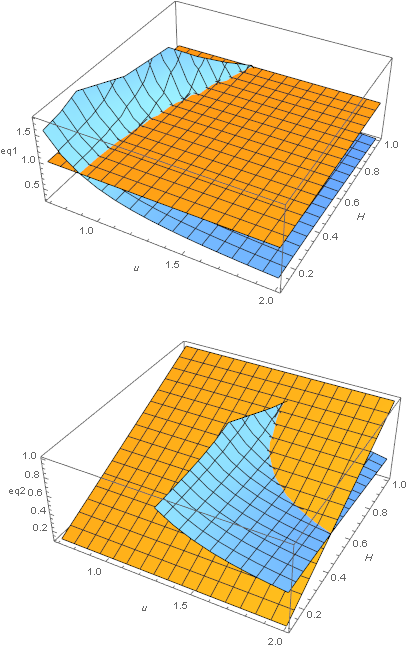
The blue area shading is the equation, the orange is the equation value. The first plot is equation 1 and the second plot is equation 2.
You can study the plot and extract values from eq1data and eq2data that show that there is no set of (u,H) values where both equations are satisfied.
If you go very far from the plotted range the equation values grow enormously.
If may well be that with different values for the input parameters there could be a root, but it appears to me that there is no root for the given parameters.
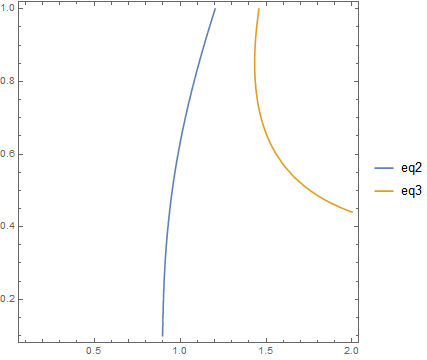
Here is a ContourPlot over the region (very slow to make).
ContourPlot[{eq1[u, H]==1, eq2[u, H]==H}, {u, 0.1, 2}, {H, 0.1, 1},
 PlotLegends -> {"eq2", "eq3"}]
This clearly shows that there is no solution for the current parameters in the region of interest.


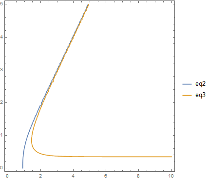
{u -> 7.30451, H -> 17.3045}, which suggests to me that you had syntax errors in your original code. Please check your edited post, copy and paste the code, and see if it works. If it does, you can use this to learn proper MMA syntax. $\endgroup$