Failure in use of SetPrecision with Filter

Question

I am working with a narrow band filter and I wish to use a high precision version. The filter is defined using Integers with Laplace variable s. Here is the, rather horrific, equation:

s =.; (* Laplace variable *)e1 = 
 1/((Cos[\[Pi]/8] - I Sin[\[Pi]/8] + (
  5000 Sqrt[
   Tan[(187 \[Pi])/10000] Tan[(193 \[Pi])/10000]] (s/(
     10000 Sqrt[
      Tan[(187 \[Pi])/10000] Tan[(193 \[Pi])/10000]]) + (
     10000 Sqrt[Tan[(187 \[Pi])/10000] Tan[(193 \[Pi])/10000]])/
     s))/(\[Pi] (-((5000 Tan[(187 \[Pi])/10000])/\[Pi]) + (
     5000 Tan[(193 \[Pi])/10000])/\[Pi]))) (Cos[\[Pi]/8] + 
  I Sin[\[Pi]/8] + (
  5000 Sqrt[
   Tan[(187 \[Pi])/10000] Tan[(193 \[Pi])/10000]] (s/(
     10000 Sqrt[
      Tan[(187 \[Pi])/10000] Tan[(193 \[Pi])/10000]]) + (
     10000 Sqrt[Tan[(187 \[Pi])/10000] Tan[(193 \[Pi])/10000]])/
     s))/(\[Pi] (-((5000 Tan[(187 \[Pi])/10000])/\[Pi]) + (
     5000 Tan[(193 \[Pi])/10000])/\[Pi]))) (-I Cos[\[Pi]/8] + 
  Sin[\[Pi]/8] + (
  5000 Sqrt[
   Tan[(187 \[Pi])/10000] Tan[(193 \[Pi])/10000]] (s/(
     10000 Sqrt[
      Tan[(187 \[Pi])/10000] Tan[(193 \[Pi])/10000]]) + (
     10000 Sqrt[Tan[(187 \[Pi])/10000] Tan[(193 \[Pi])/10000]])/
     s))/(\[Pi] (-((5000 Tan[(187 \[Pi])/10000])/\[Pi]) + (
     5000 Tan[(193 \[Pi])/10000])/\[Pi]))) (I Cos[\[Pi]/8] + 
  Sin[\[Pi]/8] + (
  5000 Sqrt[
   Tan[(187 \[Pi])/10000] Tan[(193 \[Pi])/10000]] (s/(
     10000 Sqrt[
      Tan[(187 \[Pi])/10000] Tan[(193 \[Pi])/10000]]) + (
     10000 Sqrt[Tan[(187 \[Pi])/10000] Tan[(193 \[Pi])/10000]])/
     s))/(\[Pi] (-((5000 Tan[(187 \[Pi])/10000])/\[Pi]) + (
     5000 Tan[(193 \[Pi])/10000])/\[Pi]))));

I go through the standard processes to make the filter and then apply it to some data. I do two versions one with machine precision and one with a higher precision.

sr = 5000; (* Sample rate *)
np = 50;  (* Requested precision *)
f1 = N[e1];
f2 = SetPrecision[e1, np];
tfm1 = TransferFunctionModel[{{f1}}, s];
tfm2 = TransferFunctionModel[{{f2}}, s];
dtm1 = ToDiscreteTimeModel[tfm1, 1/sr];
dtm2 = ToDiscreteTimeModel[tfm2, 1/sr];
SeedRandom[1234];
data1 = RandomReal[{-1, 1}, 1000];
SeedRandom[1234];
data2 = SetPrecision[RandomReal[{-1, 1}, 1000], np];
fdata1 = RecurrenceFilter[dtm1, data1];
fdata2 = RecurrenceFilter[dtm2, data2];

If we now examine a typical value of the machine precision and high precision versions of the output we get

fdata1[[100]]
fdata2[[100]]

A mouseover the pink box states that "No significant digits are available to display" The problem seems to come with ToDiscreteTimeModel where the imaginary part of a complex value is lost

dtm1[[1, 2, 1, 1, 1]]
dtm2[[1, 2, 1, 1, 1]]

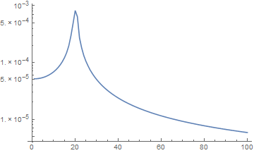
The filter in machine precision is correct as can be seen by

ft1 = Fourier[fdata1, FourierParameters -> {-1, -1}];
ListLogPlot[Abs[ft1[[1 ;; 100]]], PlotRange -> All, Joined -> True]

I thought the principle was that once a precision has been set then it should propagate through the calculations. How can I get my high precision results? (10.0 for Microsoft Windows (64-bit))

Thanks for any help.

Answer 1

This answer is entirely due to the comment from the ever helpful Daniel Lichtblau. Starting again I split the machine precision and the high precision calculations. The high precision is wrapped in a block that fixes the minimum and maximum precision. I guess that this prevents all exceptions and corrects where the precision drops to a small value.

s =.; (* Laplace variable *)e1 = 
 1/((Cos[\[Pi]/8] - I Sin[\[Pi]/8] + (
      5000 Sqrt[
       Tan[(187 \[Pi])/10000] Tan[(193 \[Pi])/10000]] (s/(
         10000 Sqrt[
          Tan[(187 \[Pi])/10000] Tan[(193 \[Pi])/10000]]) + (
         10000 Sqrt[Tan[(187 \[Pi])/10000] Tan[(193 \[Pi])/10000]])/
         s))/(\[Pi] (-((5000 Tan[(187 \[Pi])/10000])/\[Pi]) + (
         5000 Tan[(193 \[Pi])/10000])/\[Pi]))) (Cos[\[Pi]/8] + 
      I Sin[\[Pi]/8] + (
      5000 Sqrt[
       Tan[(187 \[Pi])/10000] Tan[(193 \[Pi])/10000]] (s/(
         10000 Sqrt[
          Tan[(187 \[Pi])/10000] Tan[(193 \[Pi])/10000]]) + (
         10000 Sqrt[Tan[(187 \[Pi])/10000] Tan[(193 \[Pi])/10000]])/
         s))/(\[Pi] (-((5000 Tan[(187 \[Pi])/10000])/\[Pi]) + (
         5000 Tan[(193 \[Pi])/10000])/\[Pi]))) (-I Cos[\[Pi]/8] + 
      Sin[\[Pi]/8] + (
      5000 Sqrt[
       Tan[(187 \[Pi])/10000] Tan[(193 \[Pi])/10000]] (s/(
         10000 Sqrt[
          Tan[(187 \[Pi])/10000] Tan[(193 \[Pi])/10000]]) + (
         10000 Sqrt[Tan[(187 \[Pi])/10000] Tan[(193 \[Pi])/10000]])/
         s))/(\[Pi] (-((5000 Tan[(187 \[Pi])/10000])/\[Pi]) + (
         5000 Tan[(193 \[Pi])/10000])/\[Pi]))) (I Cos[\[Pi]/8] + 
      Sin[\[Pi]/8] + (
      5000 Sqrt[
       Tan[(187 \[Pi])/10000] Tan[(193 \[Pi])/10000]] (s/(
         10000 Sqrt[
          Tan[(187 \[Pi])/10000] Tan[(193 \[Pi])/10000]]) + (
         10000 Sqrt[Tan[(187 \[Pi])/10000] Tan[(193 \[Pi])/10000]])/
         s))/(\[Pi] (-((5000 Tan[(187 \[Pi])/10000])/\[Pi]) + (
         5000 Tan[(193 \[Pi])/10000])/\[Pi]))));
sr = 5000; (* Sample rate *)
np = 50;  (* Requested precision *)
f1 = N[e1];
tfm1 = TransferFunctionModel[{{f1}}, s];
dtm1 = ToDiscreteTimeModel[tfm1, 1/sr];
SeedRandom[1234];
data1 = RandomReal[{-1, 1}, 1000];
fdata1 = RecurrenceFilter[dtm1, data1];

Block[{$MinPrecision = np, $MaxPrecision = np},
 f2 = SetPrecision[e1, np];
 tfm2 = TransferFunctionModel[{{f2}}, s];
 tfm2 = TransferFunctionModel[{{f2}}, s];
 dtm2 = ToDiscreteTimeModel[tfm2, 1/sr];
 SeedRandom[1234];
 data2 = SetPrecision[RandomReal[{-1, 1}, 1000], np];
 fdata2 = RecurrenceFilter[dtm2, data2];
 ]

This produces the messages

The example values are now all good

fdata1[[100]]
fdata2[[100]]

Thanks