Solving the magic backyard puzzle with MMA

Question

I was trying to solve this puzzle using mma

It looks like the generalization of the magic square. Anyway here my attempt:-

There are four columns $(x,y,z,w)$ and nine rowa which are denoted by the array index.

First i define the variables which have zero values

x[1] = 0; x[2] = 0; x[3] = 0; x[9] = 0; w[1] = 0;

Then the equation equating all the columns

c[1] = Sum[x[i], {i, 4, 8}];
c[2] = Sum[y[i], {i, 1, 9}];
c[3] = Sum[z[i], {i, 1, 9}];
c[4] = Sum[w[i], {i, 2, 9}];

col = Equal @@ Thread[Array[c, 4]]

Next for the rows

r[n_] := x[n] + y[n] + z[n] + w[n];
row = Equal @@ Thread[Array[r, 9]]

Here we can give some upper bound for the solutions.

all = Join[Array[x, 5, {4, 8}], Array[y, 9], Array[z, 9], Array[w, 9]];
And @@ Thread[0 <= all <= 100]

For distinct solutions:

allne = Unequal @@ 
Thread[Join[Array[x, 5, {4, 8}], Array[y, 9], Array[z, 9], 
Array[w, 8, {2, 9}]]]

List of all variables

allvar = Join[
Join[Array[x, 5, {4, 8}], Array[y, 9], Array[z, 9], 
Array[w, 8, {2, 9}]]]

Finally when I use FindInstance it just keeps running(its been 2hr now).

FindInstance[{col && row && And @@ Thread[0 <= all <= 100] && 
 allne}, allvar, Integers]

So my question is why is FindInstance so slow even after putting bounds on integer solutions.Also can this be done by any other method.

I also tried the simplest $3 \times 3$ magic square

FindInstance[
a + b + c == d + e + f == g + h + i == a + d + g == b + e + h == 
c + f + i && a != b != c != d != e != f != g != h != i, {a, b, c, 
d, e, f, g, h, i}, Integers]

This also kept on running. Do you think that i just need to wait for the output because for these kind of sums mma will take that long?

Answer 1

Another approach is to use LinearProgramming to find a configuration that satisfy the constraints. I wrote several answer illustrating some basic ideas of the method, and the use of binary decision variables ($0-1$) so I do not think it is necessary to dwell further on this topic. If necessary, you can check

• Daniel Lichtblau's answer for the "related" StackOverflow question

and my answers for

• Given a large binary matrix, find the largest submatrix containing non-zero elements
• Elegant way to partition list to be faster than ParallelTable
• Puzzle with Mathematica
• Elegant solution to the Zebra [logic] Puzzle (“Einstein's Riddle”)

Each of my answer use some "trick" to get a linear constrained optimization probelem that can be submitted to LinearProgramming, but I think the first is the one from which I would start reading.

I exploit the fact that the sum of all element cannot be less than $468$ and should be in increment of $36$. With the following function I can check if, given a set numSet of some integer numbers, there is a subset of n of these number that sums to sum.

BackyardPuzzleCheckNumberSet[numSet : {___Integer}, count_, sum_] :=
 Module[{range, m},
  range = Union@numSet; m = Length@range;
  Quiet[Check[
    Pick[range, Quiet[LinearProgramming[
       2^range,
       {range, ConstantArray[1, m]},
       {{sum, 0}, {count, 0}},
       ConstantArray[{0, 1}, m],
       Integers
       ], LinearProgramming::lpip],
     1],
    {}, LinearProgramming::lpsnf]
   ]
  ]

For example I can verify that there is a chance to fill the puzzle chart with $31$ numbers in the $0,\ldots,31$ range but not in the $1,\ldots,31$ range.

BackyardPuzzleCheckNumberSet[Range[0, 31], 31, 468]
BackyardPuzzleCheckNumberSet[Range[1, 31], 31, 468]

{0, 1, 2, 3, 4, 5, 6, 7, 8, 9, 10, 11, 12, 13, 14, 15, 16, 17, 18, 19, 20, 21, 22, 23, 24, 25, 26, 27, 29, 30, 31}

{}

This is obvious but introduce once again to LinearProgramming use and can be useful in some non-minimal scenarios. For example:

BackyardPuzzleCheckNumberSet[Range[0, 60], 31, 504]
BackyardPuzzleCheckNumberSet[Range[0, 62], 31, 112*9]

{1, 2, 3, 4, 5, 6, 7, 8, 9, 10, 11, 12, 13, 14, 15, 16, 17, 18, 19, 20, 21, 22, 23, 25, 26, 27, 28, 29, 30, 31, 32}

{17, 18, 19, 20, 21, 22, 23, 24, 25, 26, 27, 28, 29, 30, 31, 33, 34, 35, 36, 37, 38, 39, 40, 41, 42, 43, 44, 45, 46, 47, 48}

Indeed the returned list is the one with lowest numbers, so there is not chance to fill the puzzle chart with numbers that sums to $112*9$ with numbers less than $48$.

Now, to solve the puzzle, I used this function:

BackyardPuzzleTrySolve[{nr_Integer?Positive, nc_Integer?Positive}, 
  pc : {{_, _} ...}, st_Integer, numSet : {__Integer}] :=
 Module[{fp, nf, nums, nm, sr, sc, x, vars, constraints, bm, solution},
  fp = Complement[Tuples[Range /@ {nr, nc}], pc];
  nf = Length@fp;
  nums = Union@Cases[numSet, _Integer?NonNegative];
  nm = Length@nums;
  {sr, sc} = st/{nr, nc};

  vars = Flatten@Array[x, {nr, nc, nm}];
  constraints = Flatten@{
     Table[
      Sum[x[i, j, k], {k, nm}] == Boole@Not@MemberQ[pc, {i, j}], {i, 
       nr}, {j, nc}],
     Table[Sum[x[Sequence @@ ij, k], {ij, fp}] <= 1, {k, nm}],
     Table[
      Sum[nums[[k]]*x[Sequence @@ ij, k], {ij, ijl}, {k, nm}] == 
       sr, {ijl, GatherBy[fp, First]}],
     Table[
      Sum[nums[[k]]*x[Sequence @@ ij, k], {ij, ijl}, {k, nm}] == 
       sc, {ijl, GatherBy[fp, Last]}]
     };
  bm = CoefficientArrays[Equal @@@ constraints, vars];
  solution = Quiet[LinearProgramming[
     Flatten[(nums # &) /@ (2^Range[0, nr*nc - 1])],
     bm[[2]],
     Transpose@{-bm[[1]], 
       constraints[[All, 0]] /. {LessEqual -> -1, Equal -> 0, 
         GreaterEqual -> 1}},
     ConstantArray[{0, 1}, Length@vars],
     Integers
     ], {LinearProgramming::lpip, LinearProgramming::lpsnf}];

  If[Head[solution] === List,
   Partition[Extract[
     Prepend[nums, 0],
     1 + FirstPosition[#, 1, {0}] & /@ Partition[solution, nm]
     ], nc]
   , {}]
  ]

This fuction receive as input:

• the size of the grid {nr, nc}
• the list of "covered" position pc
• the expected sum st of all elements in the grid
• the set numSet of number to use (can be the result of previous function)

Just an overview of the constraints:

• every position in the grid has some number assigned iff the position is not "covered"
• every number in the list should be assigned not more than once to the "not covered" positions
• sum of positions "not covered" in each row should be st/nr
• sum of positions "not covered" in each column should be st/nc

About the cost vector (first argument of LinearProgramming): to search for any "feasible" solution you can use a null cost vector, as in many of the referenced answer. But I used a cost vector that "favor" the solutions where the lowest numbers are placed in the last (bottom-right) positions. This choice has greatly improved performances (about 2 seconds to get the solution).

So seaching for a minimal solution is:

nr = 9; nc = 4;
pc = {{1, 1}, {1, 4}, {2, 1}, {3, 1}, {9, 1}};
numSet = BackyardPuzzleCheckNumberSet[Range[0, 60], 31, 468]
BackyardPuzzleTrySolve[{nr, nc}, pc, 468, numSet] //MatrixForm // Timing
Total[sol, {1}]
Total[sol, {2}]

{117, 117, 117, 117}

{52, 52, 52, 52, 52, 52, 52, 52, 52}

and to search for a solution wher numbers sums to $504$ without using the $0$ outside of the covered positions:

numSet = BackyardPuzzleCheckNumberSet[Range[0, 60], 31, 504]
BackyardPuzzleTrySolve[{nr, nc}, pc, 504, numSet] // MatrixForm // Timing

and to search for a solution where sumbers sums to $112\times 9$

numSet = BackyardPuzzleCheckNumberSet[Range[0, 57], 31, 112*9]
BackyardPuzzleTrySolve[{nr, nc}, pc, 112*9, Range[1, 57]] // MatrixForm // Timing

Answer 2

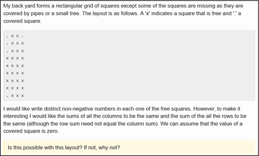
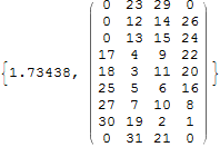
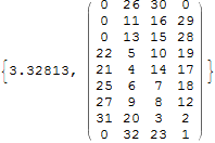
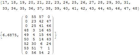
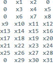
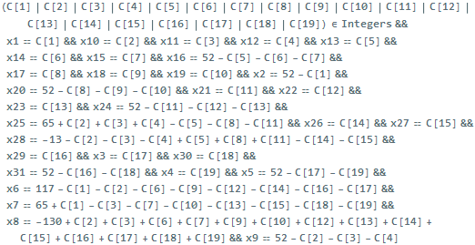
I have to post a separate answer because my approach in this one is very different from my other answer's. It is based largely on the method that Frank Kampus used here to solve a sudoku, using Backtrack from the Combinatorica package in one method, and Outer/Select in the other method. Warning: it's a long answer.

---

I managed to solve the puzzle but only through cheating by plugging in some values from the answer in this Q&A. This is because solving the puzzle from scratch took a very long time and I quit running my code after a few hours of evaluation. However, running the code with the help of the plugged in values gave the same answer as in the linked Q&A (in a matter of seconds) so I have little doubt that it will work on the original, unadulterated puzzle given enough computation resource--and patience.

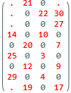
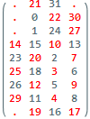
This is the matrix that I will start with. The given/cheated values are highlighted in red, and my goal now is to fill in the gray zeros you see in the matrix.

backyardCheat = {{".", 21, 0, "."}, {".", 0, 22, 30}, {".", 0, 0, 
    27}, {14, 0, 10, 0}, {0, 20, 0, 7}, {25, 0, 3, 0}, {0, 12, 0, 
    9}, {29, 0, 4, 0}, {".", 19, 0, 17}};
redHighlight[mat_List] := 
  MapAt[Style[#1, Red] &, mat, 
    Position[backyardCheat, Except[0], {2}, Heads :> False]] // MatrixForm;
backyardCheat // redHighlight

---

Step 1

For each row in the matrix, fill in the zeros of that row such that:

(1) they have to be less than or equal to 33 (VectorQ[lp, # <= 33 &]) as any higher and the total of the matrix will be greater than 468--see my other answer for why 468,

(2) all row members are different from one another (DuplicateFreeQ[lp]), and

(3) they add up to 52 (the IntegerPartitions part).

There are many permutations of each row that could satisfy both conditions, and thus an initial "sample space" (initSampleSpaceCheat) containing permutations of all 9 rows, are generated.

Clear[generateRowCheat]
generateRowCheat[l_List] :=
 Module[{whereGiven, withoutDot, countZero, partitions, perms},
  whereGiven = Select[Thread[{l, Range@4}], #1[[1]] != 0 &];
  withoutDot = DeleteCases[l, "."];
  countZero = Count[l, 0];
  partitions = 
   Cases[(Append[#, 0] & /@ 
       IntegerPartitions[52 - Total@withoutDot, {countZero - 1}])~
     Join~IntegerPartitions[52 - Total@withoutDot, {countZero}], 
    lp_List /; DuplicateFreeQ[lp] && VectorQ[lp, # <= 33 &]];
  perms = Join @@ Permutations /@ partitions;
  Fold[Insert[#1, Sequence @@ #2] &, #, whereGiven] & /@ perms
  ]

initSampleSpaceCheat = generateRowCheat /@ backyardCheat;
initSampleSpaceCheat[[8]]

As an example, above are all the permutations of the 8th row with the given values 29 in 1st place and 4 in 3rd place. As a result, the other two values will be (19, 0), (0, 19), (18, 1), and so on.

Here are the number of permutations of each row. It makes sense that less zeros there are, the less permutations as well. In fact, the rows with only one zero (1, 2, & 9) have already been filled in with the solution for that row.

Length /@ initSampleSpaceCheat
(* {1, 1, 26, 28, 26, 24, 32, 20, 1} *)

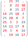
Here's a random matrix made from a single random permutation for each row:

RandomChoice[initSampleSpaceCheat[[#1]]] & /@ Range[9] // redHighlight

---

Step 2

The most glaring disqualifier for the above matrix is that even though the row values are different from one another, the column values contain duplicates. These duplicates are of two kinds:

(1) the plugged in value is a duplicate of the given value (these I call gray-red duplications, see the 14 and 25 in the first column), and

(2) two or more plugged in values are duplicates of one another (gray-gray duplications, see the 0's in the second column).

The second step will only get rid of all row permutations that lead to gray-red duplications:

---

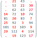
2a) Define a reference matrix. It doesn't matter what this matrix contain as long as it has all the given values and no column should contain any duplicates. The most convenient way to generate such a matrix is to plug in the positions of the zero. The indices start from 40 (to make sure that it will not be duplicate of any numbers that we will be plugging in later, whose maximum is only 33). For example, the first zero will become 43 as it is in the first row, third column.

positions = Table[ToString@i <> ToString@j // ToExpression, {i, 4, 12}, {j, 1, 4}];
givenAndPositions = MapThread[If[#1 == 0, #2, #1] &, {backyardCheat, positions}, 2];
givenAndPositions // redHighlight

---

2b) Now we can start plugging in the permutations (see ReplacePart in testQ) for each row. If a value in that row is a duplicate of a (red) given value in the same column, that permutation will be rejected (see columnQ). The result after testing all 9 rows (see /@ Range@9) will be a sample space (sampleSpace) that is smaller than the initial sample space, as evidence by taking the Length of each row in the sample space.

Clear[columnQ, testQ, sampleSpaceCheat]
columnQ[l_List] := And @@ Unequal @@@ DeleteCases[Transpose[l], ".", {2}]
testQ[n_Integer] := columnQ[ReplacePart[givenAndPositions, n :> #]] &
sampleSpaceCheat = Select[initSampleSpaceCheat[[#]], testQ[#]] & /@ Range@9;

Length /@ sampleSpaceCheat
(* {1, 1, 19, 22, 20, 18, 25, 16, 1} *)

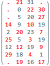
Let's make a random matrix from all the rows in sampleSpace:

RandomChoice[sampleSpaceCheat[[#1]]] & /@ Range[9] // redHighlight

---

Step 3

The above matrix now has no gray-red duplications. However, it still contains gray-gray duplication. Moreover, even if all the gray-gray duplications have been ironed out, the matrix may still contains what I called element duplications, that is, 2 numbers which are duplicates of each other, but live on 2 different rows and 2 different columns. In other words, a duplicate will not be detected if each row and column is examined, but the matrix will be invalid nonetheless. It gets worse: notice that none of the matrices you've seen so far have column sums equal to 117 (see my other answer for why this number), so we have to reject those matrices that do not meet this condition as well.

As a result, 2 tests will be applied to the current sample space:

(1) elementQ to remove element duplications--in the process, it will remove gray-gray duplications as well, and

(2) columnSumQ to remove those matrices whose columns sums are not 117.

There are 2 methods of applying these tests:

---

Method 1: Using Combinatorica package's Backtrack

The two tests mentioned above (elementQ and columnSumQ) are applied as options to Backtrack. elementQ is used to find partial solutions from the sample space, and from this partial solution space, columnSumQ will be used to arrive at the final solution.

I won't elaborate on how this works because I know nothing about this function (aside from the fact that it gives the correct solution), so someone with more knowledge on backtracking algorithms could provide some insight to this. This took less than 2 seconds to run, and the result agrees with the provided answer in the linked Q&A.

Clear[elementQ, columnSumQ, resultsBackTrackCheat]
elementQ[l_List] := Unequal @@ DeleteCases[Flatten@l, "."]
columnSumQ[l_List] := And @@ (Total[#] == 117 & /@ DeleteCases[Transpose[l], ".", {2}])    
resultsBackTrackCheat = Backtrack[sampleSpaceCheat, elementQ, elementQ[#] && columnSumQ[#] &];

redHighlight[resultsBackTrackCheat]

---

Method 2: Using Outer and Select

The difficulty of the third step compared to the second step is that now we have to test each row relative to the other rows, as opposed to testing against a static reference matrix in step 2. Hence, we rely on the use of Outer to generate various combinations of rows, and Select to reject those combinations that do not satisfy these tests.

This operation is done row-by-row, as demonstrated by this "pseudo-code":

(a) Using Outer, combine a permutation of 1st row and a permutation of 2nd row

(b) Using Select, apply test elementQ to this 2-row matrix to see if there's any element duplication

(c) If it fails the test, reject it. Otherwise, keep this 2-row matrix. (There may be several 2-row matrices that would pass elementQ.)

(d) Using Outer, combine a 2-row matrix from the last step to a permutation of the 3rd row

(e) Using Select, apply test elementQ to this 3-row matrix to see if there's any element duplication.

(f) ...

It becomes apparent that some Fold is needed to run this operation. Below is its code. Note that I define the step-wise operation twice due to a quirk of Fold when it is used to combine 2 lists (such as between the 1st and 2nd row) versus a matrix and a list (such as between the 2-row matrix and the 3rd row). The result of this operation (uniqueSolutions) are all the matrices whose elements are all different from one another.

Clear[outerSampleCheat]
(* First Fold *)
outerSampleCheat[rowSample1_?MatrixQ, rowSample2_?MatrixQ] := 
 With[{outerPermutations = Flatten[Outer[Join[{#1}, {#2}] &, rowSample1, rowSample2, 1], 1]},
  Select[outerPermutations, elementQ]]

(* Subsequent Fold's*)
outerSampleCheat[rowSamples1_List, rowSample2_?MatrixQ] := 
 With[{outerPermutations = Flatten[Outer[Join[#1, {#2}] &, rowSamples1, rowSample2, 1], 1]},
  Select[outerPermutations, elementQ]]
uniqueSoluions = Fold[outerSampleCheat, First@sampleSpaceCheat, Rest@sampleSpaceCheat];

How many of these unique-element matrices are there?

Length[uniqueSoluions]
(* 128 *)

Lastly, we will use columnSumQ to select the one matrix out of those 128 unique-element matrices whose column sums are 117.

resultsOuterSelectCheat = Select[uniqueSoluions, columnSumQ];
resultsOuterSelectCheat // First // redHighlight

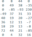
We end up with the same solution as the Backtrack method and with the correct answer:

---

The problem with solving the puzzle from scratch (optional reading)

Solving this puzzle without cheating (by plugging in some initial values) means we don't have to test the sample space against any given values i.e. skip step 2. However, this means that we end up with a giant list of permutations for each row. Moreover, we have more permutations to start with due to the presence of much more 0's in the initial matrix to be filled.

These two factors mean that the tests in step 3 will be fed a seemingly unmanageable combinations to test against, which explains their choking when I tried to solve the puzzle from scratch.

Below is the code I used to solve the puzzle from scratch. You can see that I now have much more permutations per row. Some quick calculations will indicate that there might be as much as 33!/(33 - 31)! = 4341658809405943247759097200640000000 unique-element matrices if we plug 33 different numbers into 31 slots!

Clear[backyard, generateRow, initSampleSpace, columnQ, elementQ, \
columnSumQ, outerSample]

(* Generate sample space *)
backyard = {{".", 0, 0, "."}, {".", 0, 0, 0}, {".", 0, 0, 0}, {0, 0, 
    0, 0}, {0, 0, 0, 0}, {0, 0, 0, 0}, {0, 0, 0, 0}, {0, 0, 0, 
    0}, {".", 0, 0, 0}};
generateRow[l_List] :=
  Module[{countZero, partitions, perms, whereDot},
   countZero = Count[l, 0];
   partitions = 
    Cases[(Append[#, 0] & /@ IntegerPartitions[52, {countZero - 1}])~
      Join~IntegerPartitions[52, {countZero}], 
     lp_List /; DuplicateFreeQ[lp] && VectorQ[lp, # <= 33 &]];
   perms = Join @@ Permutations /@ partitions;
   whereDot = Thread[{".", Position[l, "."]}];
   Fold[Insert[#1, Sequence @@ #2] &, #, whereDot] & /@ perms];
initSampleSpace = generateRow /@ backyard;
Length /@ initSampleSpace;
(*{14, 810, 810, 17904, 17904, 17904, 17904, 17904, 810}*)

(* Tests *)
columnQ[l_List] := 
  And @@ Unequal @@@ DeleteCases[Transpose[l], ".", {2}];
elementQ[l_List] := Unequal @@ DeleteCases[Flatten@l, "."];
columnSumQ[l_List] := And @@ (Total[#] == 117 & /@ DeleteCases[Transpose[l], ".", {2}]);

(* First Fold with Outer & Select*)
outerSample[rowSample1_?MatrixQ, rowSample2_?MatrixQ] := 
  With[{outerPermutations = 
     Flatten[Outer[Join[{#1}, {#2}] &, rowSample1, rowSample2, 1], 1]},
   Select[outerPermutations, elementQ]];
(* Subsequent Fold's with Outer & Select *)
outerSample[rowSamples1_List, rowSample2_?MatrixQ] := 
  With[{outerPermutations = 
     Flatten[Outer[Join[#1, {#2}] &, rowSamples1, rowSample2, 1], 1]},
   Select[outerPermutations, elementQ]];

And the codes to run the selection. Only run them if you have couple hours to waste!

Clear[resultsBackTrack]
resultsBackTrack = Backtrack[initSampleSpace, elementQ, elementQ[#] && columnSumQ[#] &];
Clear[resultsOuterSelect]
resultsOuterSelect = Select[Fold[outerSample, First@initSampleSpace, Rest@initSampleSpace], columnSumQ];

---

So there it is! If anyone has any idea how to optimize the process I'd greatly appreciate your effort. Big thanks for Mr. Frank Kampus for his very readable walkthrough of solving a related problem (the sudoku); all credits should go to him for this is all his ideas.

Answer 3

Below is my (unsuccessful) attempt at solving the problem. I think this is an interesting problem that the MMA experts on here could help solve, and in the process will hopefully reveal the capabilities of MMA.

1) I borrowed from the answer in the linked Q&A the fact that the total of all elements in the matrix will be 468.

This means that the row and column sums are divisors of 468. Moreover, these sums have to be related to each other by a factor of 9/4 (or 4/9). With that information, I picked out the possible candidates for those sums out of the divisors of 468.

Cases[Divisors[468],x_/;Or@@(MemberQ[#,x]&/@{#*9/4,#*4/9}&@Divisors[468])]
(* {4,9,52,117} *)

4 and 9 are too small to be sums. Therefore, the row sum has to be 52 and the column sum has to be 117.

2) This is the 9-by-4 garden with the different variables:

garden={{0,x1,x2,0},{0,x3,x4,x5},{0,x6,x7,x8},{x9,x10,x11,x12},{x13,x14,x15,x16},{x17,x18,x19,x20},{x21,x22,x23,x24},{x25,x26,x27,x28},{0,x29,x30,x31}};

vars=Variables[garden]

3) We construct 9 row sum equations and 4 column sum equations:

rowEqns=And@@(Total[garden[[#1]]]==52&/@Range@Length@garden)

columnEqns=And@@(Total[garden[[All,#1]]]==117&/@Range@Length@Transpose@garden)

4) Use Reduce to solve all sum equations (see end for some sidenotes):

reduced=Reduce[And[rowEqns,columnEqns],vars,Integers]

The 31-variable equations now become 19-variable (the rest dependent variable). It's not the ideal solution but let's work with it.

5) Generate non-repeating values of C[1] to C[19] and plug that into the reduced solution:

randomC=Thread[C[#]&/@Range@19:>Evaluate@RandomSample[Range@52,19]];

randomx=Rest@reduced/.randomC/.{And->List,Equal->Rule}

gardenFilled=garden/.randomx;

This is where I gave up for now, as even though the column and row lengths all add it to the correct values (52 for row, 117 for column), there are negative values. Moreover, there's no guarantee that the other values aside from C[1] to C[19] will be unique.

One idea for post-processing the reduced solution is to NestWhile with a different random samples of C[1] to C[19] until there are (1) no negative values, and (2) no repeating values, but I'd wasted enough time today working on this problem. Perhaps I could work on it some time later or someone else could arrive at the solution before then.

Lastly, the answer in the linked Q&A mentioned a backtracking algorithm to arrive at his/her solution. I'm not advanced enough to implement one in MMA so perhaps someone with knowledge in that area could think of a method to solve the problem.

*

I also tried to impose all kinds of conditions on the variables, such as:

a) They have to be positive

positiveCond=And@@(#>=0&/@vars)

b) They have to be less than 52

lessCond=And@@(#<52&/@vars)

, or c) They have to be different from one another

diffCond=Unequal@@Variables[garden]

, but they had been nothing but making the Reduce run forever.

reduced = Reduce[And[rowEqns, columnEqns, diffCond], vars, Integers]

:(