0
$\begingroup$

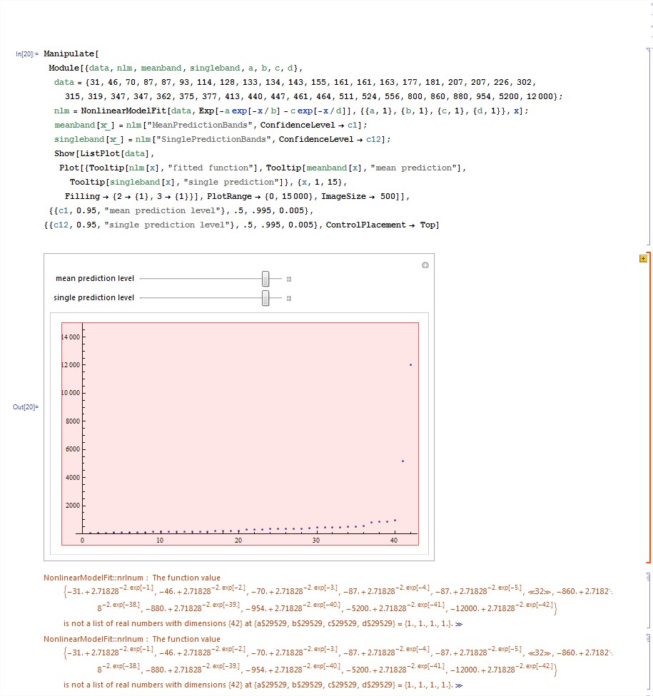
I am trying to fit a double exponential curve to my data, but I got the error saying there are non real number.

Also I tried with starting values for my 4 parameters, but this does not work either.

I'm doing my tries by modifing this CDF: http://demonstrations.wolfram.com/MeanAndSinglePredictionBandsForANonlinearModel/

And my code and extreme data are these:

Manipulate[
 Module[{data, nlm, meanband, singleband, a, b, c, d},

  data = {31, 46, 70, 87, 87, 93, 114, 128, 133, 134, 143, 155, 161, 
    161, 163, 177, 181, 207, 207, 226, 302, 315, 319, 347, 347, 362, 
    375, 377, 413, 440, 447, 461, 464, 511, 524, 556, 800, 860, 880, 
    954, 5200, 12000};

  nlm = NonlinearModelFit[data, 
    Exp[-a Exp[-x/b] - c Exp[-x/d]], {{a, 1}, {b, 1}, {c, 1}, {d, 1}},
     x]; 
  meanband[x_] = nlm["MeanPredictionBands", ConfidenceLevel -> c1];
  singleband[x_] = nlm["SinglePredictionBands", ConfidenceLevel -> c12];

  Show[ListPlot[data],
     Plot[{Tooltip[nlm[x], "fitted function"], 
     Tooltip[meanband[x], "mean prediction"],
     Tooltip[singleband[x], "single prediction"]}, {x, 1, 15},
    Filling -> {2 -> {1}, 3 -> {1}}], PlotRange -> {0, 15000}, 
   ImageSize -> 500]],
 {{c1, 0.95, "mean prediction level"}, .5, .995, 0.005},
 {{c12, 0.95, "single prediction level"}, .5, .995, 0.005}, 
 ControlPlacement -> Top]

What could I do to fix this error? enter image description here

$\endgroup$
2
  • 6
    $\begingroup$ I would change exp to Exp in the first place :) $\endgroup$
    – eldo
    Commented Jul 17, 2014 at 21:00
  • $\begingroup$ Thanks you eldo. Now it works, although I only see half mean confidence or prediction band, not the single prediction band nor the fitted curve (cumulative frequency or CFD). Also, this is the data of a time series, but now I think I have to obtain the cumulative observed CFD and then to apply the data of the published example. $\endgroup$
    – JosGranada
    Commented Jul 18, 2014 at 11:10

2 Answers 2

2
$\begingroup$

I don't think this is a general answer, but the error you are getting is related to the nonlinear least squares regression in your Module. You can get rid of the error by constraining your optimization. Using the default methods of NonlinearModelFit and placing the following restrictions on the parameters $b$ and $c$, as well as suppressing warning in the bound calculations with Quiet, you can rewrite the method as

    Manipulate[
     Module[{data, nlm, meanband, singleband, a, b, c, d}, 
      data = {31, 46, 70, 87, 87, 93, 114, 128, 133, 134, 143, 155, 161, 
        161, 163, 177, 181, 207, 207, 226, 302, 315, 319, 347, 347, 362, 
        375, 377, 413, 440, 447, 461, 464, 511, 524, 556, 800, 860, 880, 
        954, 5200, 12000};
      nlm = NonlinearModelFit[
        data, {Exp[-a Exp[-x/b] - c Exp[-x/d]], b > 1, 
         d > 1}, {{a, 1}, {b, 1}, {c, 1}, {d, 1}}, x];
      meanband[x_] = 
       Quiet@nlm["MeanPredictionBands", ConfidenceLevel -> c1];
      singleband[x_] = 
       Quiet@nlm["SinglePredictionBands", ConfidenceLevel -> c12];
      Show[ListPlot[data], 
       Plot[{Tooltip[nlm[x], "fitted function"], 
         Tooltip[meanband[x], "mean prediction"], 
         Tooltip[singleband[x], "single prediction"]}, {x, 1, 
         Length[data]}, Filling -> {2 -> {1}, 3 -> {1}}, 
        PlotRange -> All], PlotRange -> {0, 15000}, 
       ImageSize -> 500]], {{c1, 0.95, "mean prediction level"}, .5, .995,
       0.005}, {{c12, 0.95, "single prediction level"}, .5, .995, 0.005}, 
     ControlPlacement -> Top]

While this appears to fix the error message you were previously receiving, the default methods of NonlinearModelFit don't appear to converge for a reasonable starting points and number of iterations. You can live with this fitting, suppressing the warning with Quiet by substituting the following in the Module definition:

    nlm = Quiet@NonlinearModelFit[data, {Exp[-a Exp[-x/b] - c Exp[-x/d]], 
      b > 1, d > 1}, {{a, 1}, {b, 1}, {c, 1}, {d, 1}}, x];

This method gives something to the effect of
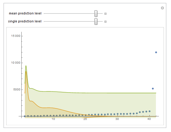
Default fitting methods

I was able to improve the fitting of the model by using an alternative Method in NonlinearModelFit. The following post provides a great introduction to nonstandard methods in NonlinearModelFit. Using the DifferentialEvolution method of NMinimize, the function can now be constructed as

    Manipulate[
     Module[{data, nlm, meanband, singleband, a, b, c, d}, 
      data = {31, 46, 70, 87, 87, 93, 114, 128, 133, 134, 143, 155, 161, 
        161, 163, 177, 181, 207, 207, 226, 302, 315, 319, 347, 347, 362, 
        375, 377, 413, 440, 447, 461, 464, 511, 524, 556, 800, 860, 880, 
        954, 5200, 12000};
      nlm = NonlinearModelFit[
        data, {Exp[-a Exp[-x/b] - c Exp[-x/d]], b > 1, 
         d > 1}, {{a, 1}, {b, 1}, {c, 1}, {d, 1}}, x, 
        Method -> {NMinimize, 
          Method -> {"DifferentialEvolution", "ScalingFactor" -> 0.9, 
            "CrossProbability" -> 0.1, "SearchPoints" -> 50, 
            "PostProcess" -> {FindMinimum, Method -> "QuasiNewton"}}}];
      meanband[x_] = 
       Quiet@nlm["MeanPredictionBands", ConfidenceLevel -> c1];
      singleband[x_] = 
       Quiet@nlm["SinglePredictionBands", ConfidenceLevel -> c12];
      Show[ListPlot[data], 
       Plot[{Tooltip[nlm[x], "fitted function"], 
         Tooltip[meanband[x], "mean prediction"], 
         Tooltip[singleband[x], "single prediction"]}, {x, 1, 
         Length[data]}, Filling -> {2 -> {1}, 3 -> {1}}, 
        PlotRange -> All], PlotRange -> {0, 15000}, 
       ImageSize -> 500]], {{c1, 0.95, "mean prediction level"}, .5, .995,
       0.005}, {{c12, 0.95, "single prediction level"}, .5, .995, 0.005}, 
     ControlPlacement -> Top]

There is a bunch of information on global numerical optimization in Mathematica here. There are a variety of options available in Method for both NonlinearModelFit, as well as NMinimize. Using this modified optimization technique in NonlinearModelFit, the function now yields:
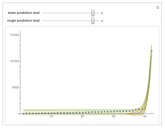
enter image description here

$\endgroup$
2
$\begingroup$

Maybe this is just an extended comment but I think the answer is to consider a different function to fit.

First, you should consider a "single exponential" by taking the log of the dependent variable and the "double exponential":

data = Log[{31, 46, 70, 87, 87, 93, 114, 128, 133, 134, 143, 155, 161,
     161, 163, 177, 181, 207, 207, 226, 302, 315, 319, 347, 347, 362, 
    375, 377, 413, 440, 447, 461, 464, 511, 524, 556, 800, 860, 880, 
    954, 5200, 12000}];

nlm = NonlinearModelFit[data, 
   a Exp[-x/b] + c Exp[-x/d], {{a, 1}, {b, 1}, {c, 1}, {d, 1}}, x];
nlm["BestFitParameters"]
(* {a -> -1.67415*10^7, b -> 1.21231*10^8, c -> 1.67415*10^7, d -> 2.94828*10^8} *)
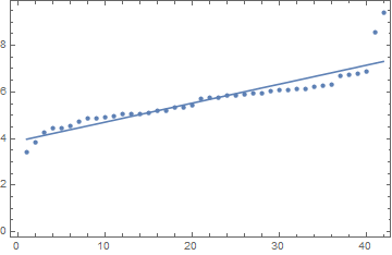
Show[ListPlot[data], Plot[nlm[x], {x, 1, Length[data]}], Frame -> True]

Data and fit

There is considerable "lack-of-fit". Also, if WorkingPrecision and MaxIterations are increased from the default, then all of the coefficients get larger and larger in absolute value but ending up with essentially the same (poor) fit.

How did the form of the double exponent come to be? Is there some theoretical reason?

$\endgroup$

Your Answer

By clicking “Post Your Answer”, you agree to our terms of service and acknowledge you have read our privacy policy.

Not the answer you're looking for? Browse other questions tagged or ask your own question.