Numerical Instability?

Question

Current Status

Please skip ahead to Update 2: the key questions are now:

1/ Why does Mma generally fail to find the minimum for a well behaved function when the function does not have infinite precision but the specified precision seems more than sufficient to the task

2/ Why does Mma fail to find the minimum when the precision of calculations is increased beyond the point at which it is first able to minimise the function

The original question need only be consulted for background, if desired.

End Current Status

Further to this initial question on controlling precision and with the benefit of rasher & Mr Wizard's (previous) input I now have control over my calculation precision (I think, but I am still very much a beginner so I beg your collective indulgence...).

However, the results are wildly unstable as I increase precision, though to my eyes the equations look well-behaved in the regions of interest. I only took an interest in the precision when the machine precision results did not seem physically reasonable.

I am seeking maxima and minima for four variables, t, x, y & z and have - I think - good reason (see separate section below) to believe that for x, y, and z the minima should be equal, and so should the maxima.

What I find for ~machine precision is (focussing on the minima only):

x = -0.222222222222222
y = -1.242253153494817
z = -1.222222222222222

These are clearly unequal with differences of the same magnitude as the values. (NB. When 3D plotting the resulst of the tranformations, these erroneous values lead to the transformed sphere being truncated when the plot range is determined in terms of these extrema, so when Mma is plotting the equations it is generating values significantly different to those it comes up with during minimization etc.]

With precision set to 50 the results are very different:

x = -1.2619796324000608024205195519983014313647470787550
y = -1.2619796324000608024205195519983014313647470787550
z = -1.2619796324000608024205195519983014313647470787550

Clearly these three are identical to the specified precision, but increase it further to 100 and one obtains

x = -1.261979632400060802420519551998301431364747078755025069028958918198601669661636873543419739259161731
y = -1.261979632400060802420519551998301431364747078755025069028958918198601669661636873543419739259161731
z = -1.222222222222222222222222222222222222222222222222222222222222222222222222222222222222222222222222222

Now x = y still, and the results agree with the previous output to 50 digits, but z has changed in the 2nd decimal place.

There are of course similar problems with the maxima - and it should be noted that the maxima probably ought to have the same magnitudes as the minima, which they don't.

Can anyone explain what is going on and how can I reliably estimate the desired minima and maxima?

Code

Note also the output of the MinValue function... as an incidental question, why does it not achieve the same prevision as Minimize?

(Thanks to belisarius for prettifying the code)

To the best of my knowledge the equations are correct for the physics.

$PreRead = (# /. s_String /; StringMatchQ[s, NumberString] && 
        Precision@ToExpression@s == MachinePrecision :>   s <> "`100." &);
Block[{γ, vx, vy, vz, t0, x0, y0, z0, t1},
 t0 = γ (t1 - vx Sin[θ] Sin[ϕ] - vy Cos[θ] Sin[ϕ] - vz Cos[ϕ]);
 x0 = (-γ t1 vx - γ^2 t1 vx +    Sin[θ] Sin[ϕ] + γ Sin[θ] Sin[ϕ] + 
      γ^2 vx^2 Sin[θ] Sin[ϕ] + γ^2 vx vy Cos[θ] Sin[ϕ] + γ^2 vx vz Cos[ϕ])/(1 + γ);
 y0 = ((1 + γ + γ^2 vy^2) Cos[θ] Sin[ϕ] - γ vy (t1 + γ t1 - γ vx Sin[θ] Sin[ϕ]) + 
      γ^2 vy vz Cos[ϕ])/(1 + γ);
 z0 = (γ vz (-(1 + γ) t1 + γ vx Sin[θ] Sin[ϕ] + γ vy Cos[θ] Sin[ϕ]) + 
      (1 + γ + γ^2 vz^2) Cos[ϕ])/(1 + γ);
 vx = vy = vz = 0.8/Sqrt[3]; 
 γ = 1/Sqrt[1 - (vx^2 + vx^2 + vx^2)]; 
 Print["γ = ", γ];
 t1 = 0;
 Print["Precision of t0 = ", Precision[t0], " of x0 = ", 
        Precision[x0], " of y0 = ", Precision[t0], " of t0 = ", Precision[z0]];
 Print["Precision of Cos[ϕ] = ", Precision[Cos[ϕ]]];
 Print["MinValue of t0 = ", MinValue[{t0, 0. <= θ < 2 Pi, -Pi <= ϕ <= Pi}, {θ, ϕ}, Reals]] ;
 Print[{Minimize[{t0, 0 <= θ < 2 Pi, -Pi <= ϕ < Pi}, {θ, ϕ}, Reals], 
       Maximize[{t0, 0 <= θ < 2 Pi, -Pi <= ϕ < Pi}, {θ, ϕ},  Reals]}];
 Print[{Minimize[{x0, 0 <= θ < 2 Pi, -Pi <= ϕ < Pi}, {θ, ϕ}, Reals], 
       Maximize[{x0, 0 <= θ < 2 Pi, -Pi <= ϕ < Pi}, {θ, ϕ},  Reals]}];
 Print[{Minimize[{y0, 0 <= θ < 2 Pi, -Pi <= ϕ < Pi}, {θ, ϕ}, Reals], 
       Maximize[{y0, 0 <= θ < 2 Pi, -Pi <= ϕ < Pi}, {θ, ϕ},  Reals]}];
 Print[{Minimize[{z0, 0 <= θ < 2 Pi, -Pi <= ϕ < Pi}, {θ, ϕ}, Reals], 
        Maximize[{z0, 0 <= θ < 2 Pi, -Pi <= ϕ < Pi}, {θ, ϕ}, Reals]}];
 ]

Reasons to believe extrema should be equal

The equations given in the code sample describe the Lorentz transformation of a sphere from one frame of reference to another. For simplicity, albeit in the general case, the sphere is moving with equal velocity in all three spatial directions. As is well known, according to Special Relativity the sphere should be contracted along the direction of motion - in this case in the direction {1,1,1}. Consequently by symmetry of the sphere and equality of motion with respect to x, y, z, the x, y, z minima (the coordinate distances to the "back" of the sphere, assuming it is moving away) should all be the same. Likewise for the maxima. The fact that the sphere is defined in terms of parametric equations in polar coordinates (SinSin, CosSin and Cos) obscures this, but again by symmetry the orientation of the axes in the sphere's rest frame shouldn't make any difference either.

The fact that the x, y, z extrema are bigger and not smaller than 1 (sphere radius) is due to the fact that they are the transformed values in the other frame and are not simultaneous, so do not represent the Lorentz contraction directly: what is actually being calculated here is the spatial envelope over time in the other frame.

Update

I have tried to apply MichaelE2's "uncertainty" function given in answer to another question here and obtain the following results (focusing on z0 only for brevity).

Adding the following code to that already given (declare extra block vars as necessary - as noted in chat, I have been unable to get the M.SE toolbar to work for me, so apologies for the γ, etc. again)

minz = Minimize[{z0, 
   0 <= θ < 2 Pi, -Pi <= ϕ < Pi}, {θ, ϕ}, 
  Reals]; maxz = 
 Maximize[{z0, 
   0 <= θ < 2 Pi, -Pi <= ϕ < Pi}, {θ, ϕ}, 
  Reals];
(* unset all variables again so that uncertainty can take the \
derivative... *)
vx =. ; vx =.; vz =.; γ =.; t1 =.;
Print[minz[[2, 1]], maxz[[2, 2]]];
Print["Uncertainty in min z0 = ", 
  uncertainty[
   z0  /.  γ -> 1/Sqrt[1 - (vx^2 + vy^2 + vz^2)], {minz[[2, 
     1]], minz[[2, 2]], vx -> 0.8/Sqrt[3], vy -> 0.8/Sqrt[3], 
    vz -> 0.8/Sqrt[3], t1 -> 0}]];

I obtain

for precision =  20, Uncertainty in min z0 = 4.61791*10^-20
              =  50, Uncertainty in min z0 = 8.63608*10^-50
              = 100, Uncertainty in min z0 = 4.55654*10^-100

This suggests to me, naively perhaps!, that the answers previously given should have agreed to the precision specified, and since they did not I remained baffled as to what is going on.

Update 2 (21 Mar) - the plot thickens

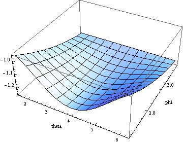
Summary: having had my attention drawn to the form of z0 by @MichelE2's comment an error was detected: phi, which is a spherical polar coordinate was running from -Pi to Pi, instead of 0 to Pi, which created double minima. Corrected, there is now only one minimum, as this plot of z0 shows nicely

We now find that if z0 has infinite precision, Minimize solves analytically and N[] of the solutions can be obtained to specified precision - and the answers agree with the application of NMinimize [why are the specs for those functions so different???]

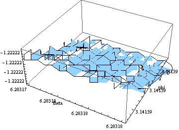
However... we also find that subjecting the variables to careful precision control, both Minimize and NMinimize fail to find the correct answer unless prec = 45 to 47. It can be seen that they are getting stuck in the corner at phi = Pi, which for the well behaved function z0 does not seem reasonable. Automatic plotting of the region of interest fails (plot range min and max become the same) but a manual plot range shows this

which doesn't look nice at all. [NB note that I have tweaked WorkingPrecision to keep it at least consistent with prec]

Given the reasonable behaviour of z0, what is the reason that Mma is generally unable to (N)Minimize[z0] and when precision has "increased enough" to do it, how can it fail again at higher precision.

This does not seem right at all.

Code for this update follows...

Block[{γ, vx, vy, vz, t0, prec, mint, maxt, minx, maxx, miny, 
  maxy, minz, maxz, K, plotMinTheta, plotMinPhi, },
 z0 = (γ vz (-(1 + γ) t1 + γ vx Sin[θ] \
Sin[ϕ] + γ vy Cos[θ] Sin[ϕ]) + (1 + γ \
+ γ^2 vz^2) Cos[ϕ])/(1 + γ);
 prec = 44; K = 8/10; 
 t1 = 0; (* prec = 45 to 47 is 1st range for which part 2 gives \
correct answer, then from 103 to..? *)
 vx = vy = vz = (8/10)/Sqrt[3]; γ = 
  1/Sqrt[1 - (vx^2 + vx^2 + vx^2)]; t1 = 0;
 Print["For precision of t1 = ", Precision[t1], ", of K = ", 
  Precision[K], ", of γ = ", Precision[γ], ", of z0 = ",
   Precision[z0]];
 minz = Minimize[{z0, 0 <= θ < 2 Pi, 
    0 <= ϕ < Pi}, {θ, ϕ}, Reals];
 plotMinTheta = N[2 (  θ - Pi) /. minz[[2]][[1]], prec]; 
 plotMinPhi = 
  N[(2 ϕ - Pi) /.  minz[[2]][[2]], 
   prec]; (* to centre the minimum found *)
 Print["N[Min,$MachinePrecision,] = ", N[minz, $MachinePrecision]];
 Print["N[Min,", prec, "] = ", N[minz, prec]];
 Print["NMinimize[z0] = ", 
  NMinimize[{z0, 0 <= θ < 2 Pi, 
    0 <= ϕ < Pi, θ ∈ Reals, ϕ ∈ 
     Reals}, {θ , ϕ}, WorkingPrecision -> (89/100)*prec, 
   MaxIterations -> 200]]; 
 Print[Plot3D[
   z0, {θ, plotMinTheta, 2 Pi}, {ϕ, plotMinPhi, Pi}, 
   PlotRange -> Automatic,  AxesLabel -> {"theta", "phi"}, 
   WorkingPrecision -> (89/100)*prec, Mesh -> 10]];

 vx = vy = vz = N[K, prec]/Sqrt[3]; γ = 
  1/Sqrt[1 - (vx^2 + vx^2 + vx^2)]; t1 = 0;
 Print["For precision of t1 = ", Precision[t1], ", of K = ", 
  Precision[K], ", of γ = ", Precision[γ], ", of z0 = ",
   Precision[z0]];
 Print["NMinimize[z0] = ", 
  NMinimize[{z0, 0 <= θ < 2 Pi, 
    0 <= ϕ < Pi, θ ∈ Reals, ϕ ∈ 
     Reals}, {θ , ϕ}, WorkingPrecision -> (89/100)*prec]]; 
 minz = Minimize[{z0, 0 <= θ < 2 Pi, 
    0 <= ϕ < Pi}, {θ, ϕ}, Reals]; 
 plotMinTheta = N[2 (  θ - Pi) /. minz[[2]][[1]], prec]; 
 plotMinPhi = 
  N[(2 ϕ - Pi) /.  minz[[2]][[2]], 
   prec]; (* depending on prec, will not work when phi of minimum \
\[Equal] Pi ! *)
 Print["N[Minimize[z0],", prec, "] = ", N[minz, prec]];
 Print[Plot3D[
   z0, {θ, plotMinTheta, 2 Pi}, {ϕ, plotMinPhi, Pi}, 
   PlotRange -> Automatic,  AxesLabel -> {"theta", "phi"}, 
   WorkingPrecision -> (89/100)*prec, Mesh -> 10]];
 Print[Plot3D[
   z0, {θ, N[6.28317, prec], 2 Pi}, {ϕ, 0.999999 Pi, Pi}, 
   PlotRange -> Automatic, AxesLabel -> {"theta", "phi"}, 
   WorkingPrecision -> (89/100)*prec, Mesh -> 10]];
 ]

Answer 1

Global optimization is (mathematically speaking) hard. There's no guaranteed way to find the maximum or minimum. You might read this tutorial -- a cursory reading is enough to convince one that optimization is complicated. The biggest problem is simply that unless you can find all the critical points, there is no way to be certain that a local extremum is a global one.

Nonetheless the functions and their derivatives are relatively simple, simple enough for Mathematica's solvers to find all the critical points. Looking for the exact solution is well within their reach and only takes a few seconds.

results = Block[{γ, vx, vy, vz, t0, x0, y0, z0, t1}, 
   t0 = γ (t1 - vx Sin[θ] Sin[ϕ] - 
       vy Cos[θ] Sin[ϕ] - vz Cos[ϕ]);
   x0 = (-γ t1 vx - γ^2 t1 vx + 
       Sin[θ] Sin[ϕ] + γ Sin[θ] Sin[ϕ] + γ^2 vx^2 Sin[θ] Sin[ϕ] +
        γ^2 vx vy Cos[θ] Sin[ϕ] + γ^2 vx vz Cos[ϕ])/(1 + γ);
   y0 = ((1 + γ + γ^2 vy^2) Cos[θ] Sin[ϕ] -
       γ vy (t1 + γ t1 - γ vx Sin[θ] Sin[ϕ]) + γ^2 vy vz Cos[ϕ])/(1 + γ);
   z0 = (γ vz (-(1 + γ) t1 + γ vx Sin[θ] Sin[ϕ] + γ vy Cos[θ] Sin[ϕ]) +
       (1 + γ + γ^2 vz^2) Cos[ϕ])/(1 + γ);
   vx = vy = vz = 8/10/Sqrt[3];(******)
   γ = 1/Sqrt[1 - (vx^2 + vx^2 + vx^2)];
   t1 = 0;
   {Minimize[{t0, 0 <= θ < 2 Pi, -Pi <= ϕ < Pi}, {θ, ϕ}, Reals],
    Minimize[{x0, 0 <= θ < 2 Pi, -Pi <= ϕ < Pi}, {θ, ϕ}, Reals],
    Minimize[{y0, 0 <= θ < 2 Pi, -Pi <= ϕ < Pi}, {θ, ϕ}, Reals],
    Minimize[{z0, 0 <= θ < 2 Pi, -Pi <= ϕ < Pi}, {θ, ϕ}, Reals]
    }
   ];
N[results]
(*
  {{-1.33333, {θ -> 0.785398, ϕ -> 0.955317}},
   {-1.26198, {θ -> 4.53254,  ϕ -> 1.74781}},
   {-1.26198, {θ -> 3.32145,  ϕ -> 1.74781}},
   {-1.26198, {θ -> 0.785398, ϕ -> -2.88991}}}
*)

One can see the pitfalls below :) in using numerical optimization for this problem. There are three local minima for y0 and z0. I do not know the specifics of the implementations to say why the optimization routines get trapped in one basin or another depending on precision. NMinimize methods let you specify initial points, when numerical methods are preferred. One could start near the local minima and let NMinimize sort out the global minimum. See the tutorial linked above. FindMinimum requires a starting point, and one could apply it to a number of starting points separately, if you knew the approximate locations of the critical points.

plots = Block[{γ, vx, vy, vz, t0, x0, y0, z0, t1}, 
   t0 = γ (t1 - vx Sin[θ] Sin[ϕ] - vy Cos[θ] Sin[ϕ] - vz Cos[ϕ]);
   x0 = (-γ t1 vx - γ^2 t1 vx + 
       Sin[θ] Sin[ϕ] + γ Sin[θ] Sin[ϕ] + γ^2 vx^2 Sin[θ] Sin[ϕ] +
        γ^2 vx vy Cos[θ] Sin[ϕ] + γ^2 vx vz Cos[ϕ])/(1 + γ);
   y0 = ((1 + γ + γ^2 vy^2) Cos[θ] Sin[ϕ] -
         γ vy (t1 + γ t1 - γ vx Sin[θ] Sin[ϕ]) + γ^2 vy vz Cos[ϕ])/(1 + γ);
   z0 = (γ vz (-(1 + γ) t1 + γ vx Sin[θ] Sin[ϕ] + γ vy Cos[θ] Sin[ϕ]) +
         (1 + γ + γ^2 vz^2) Cos[ϕ])/(1 + γ);
   vx = vy = vz = (8/10)/Sqrt[3];
   γ = 1/Sqrt[1 - (vx^2 + vx^2 + vx^2)];
   t1 = 0;
   {(*Plot3D[t0,{θ,0,2 Pi},{ϕ,-Pi,Pi}],*)
    Plot3D[x0, {θ, 0, 2 Pi}, {ϕ, -Pi, Pi}],
    Plot3D[y0, {θ, 0, 2 Pi}, {ϕ, -Pi, Pi}],
    Plot3D[z0, {θ, 0, 2 Pi}, {ϕ, -Pi, Pi}]
    }
   ];

Show[#, PlotRange -> {-1.22, -1.27}] & /@ plots