2
$\begingroup$

I have a coupled boundary ODE with dependent variables $u=u(x)$ and $z=z(x)$,

$$u'' - \frac{1}{z} \left( -3 + u'^2 (3 - c\; e^{-g u} z^4) - 6 u' z' \right) = 0\tag{1}$$

$$z'' + c\; e^{-g u} z^3 (-3 + 4 u'^2 - 2 u' z') - \frac{3}{z} \left( -1 + u'^2 - 2 u' z' \right) - c^2 e^{-2 g u} z^7 u'^2 - \frac{1}{2} c\; g\; e^{-g u} z^4 u'^2 = 0 \tag{2}$$

where the boundary conditions (B.C.) are fixed on one point $u_f(b)$, $z_f(b)$, while the other is free to move and a derivative condition is imposed,

$$u'_i(a) = \pm \sqrt{\frac{4}{1 - 4 \left(1 - c\; e^{-g u_i(a)} z_i(a)^4 \right)}}\tag{3}$$

$$z'_i(a) = \pm (1 - c\; e^{-g u_i(a)} z_i(a)^4) \sqrt{\frac{4}{1 - 4 \left(1 - c\; e^{-g u_i(a)} z_i(a)^4 \right)}}\tag{4}$$

where in the code I have squared the inside of the square root then applied another square root in order to avoid complex values since depending on how the solution converges the inside may be negative. The domain is given by $x \in [a,b]$. So, the free parameters here are $u_i(a)$ and $z_i(a)$ which we can input "guess" values to start the calculation.

I'm using finite-difference method while employing a relaxation technique to solve the boundary ODE which are eq01 and eq02 in the code.

Parameters: 0 < c < (not too large, maybe at most 10^5) and g is a damping factor which as can be seen is in the exponent; a b zf uf are fixed; n is the number of grid points while h is the grid size; zi ui can be changed so as to lead to convergence.

Procedure (I think this is not necessary to know to understand the issue): I have built a sparse matrix where the free B.C. is on the upper left and the fixed B.C. is on the lower right. resid indicates the residual of the finite-difference not on the boudary while residbound indicates the residual of the boundary. The sparse matrix sparse was constructed, then a relaxation technique was employed with iteration m and relaxation parameter 0 < w < 1; w can be changed for faster convergence and m can be increased for smaller error. In addition, initial values represented by init[0] were injected (it includes the aforementioned ui zi). The matrix DFxmat and the vector Residvec are the sparse matrix and residual vector where inputs were injected.

The issue: Given the matrix DFxmat and the vector Residvec, I used LinearSolve to compute the solution. However, it gives an error saying that DFxmat is badly conditioned. One check that can be done if it is rank deficient, probably due to very small numbers is to calculate MatrixRank = 200 which is the same as the size of the matrix so it is not deficient. However, the condition number gives a really large value ConditionNumber = 10^11. One thing I'm thinking about is maybe it is due to a large difference in the entries of the matrix where some entries could be of order $10^0$ while others are $10^6$. Changing w to some other number may not give a warning error but the ConditionNumber is still big, in addition it still does not give a satisfactory solution (see Addendum). Overall, I'm not sure what is contributing to this issue and I don't know how to resolve this.

Addendum: The solution that I want should give a residual error of order $10^{-10}$ or at least close. However, the issue is giving an error of $\sim 0.26$. I know that by increasing the grid points n a better approximation can be achieved, but for the purposes of the issue I just set it to n=100.

(*Two Coupled ODE Setup*)
Clear["Global`*"]
Needs["VariationalMethods`"]
c = 1000;
g = 3;
m = c Exp[-g u[x]];
f = 1 - m z[x]^(d + 1);
L = Sqrt[-f u'[x]^2 + 2 u'[x] z'[x] + 1]/z[x]^d;
eq1 = EulerEquations[L, u[x], x];
eq2 = EulerEquations[L, z[x], x];
s = Solve[{eq1, eq2} /. d -> 3, {u''[x], z''[x]}][[1]] // Simplify;
eq01 = u''[x] - s[[1, 2]];
eq02 = z''[x] - s[[2, 2]];

(*Parameters*)
n = 100;
h = (b - a)/(n - 1);
a = 0;
b = 10^-2;
zf = 10^-2;
uf = 0.03;
ui = 0.1;
zi = 0.26;
up = Sqrt[Sqrt[((d - 1)^2/(1 - (d - 1)^2 (1 - c Exp[-g u[1]] (z[1])^(d + 1))))^2]] /. d -> 3;
zp = -(1 - c Exp[-g u[1]] (z[1])^(d + 1)) Sqrt[Sqrt[((d - 1)^2/(1 - (d - 1)^2 (1 - c Exp[-g u[1]] (z[1])^(d + 1))))^2]] /. d -> 3;

(*Sparse Matrix Setup*)
rule = {u''[x] -> ((u[i + 1] - 2 u[i] + u[i - 1])/h^2), u'[x] -> ((u[i + 1] - u[i - 1])/(2 h)), u[x] -> u[i], z''[x] -> ((z[i + 1] - 2 z[i] + z[i - 1])/h^2), z'[x] -> ((z[i + 1] - z[i - 1])/(2 h)), z[x] -> z[i]};
resid1 = h^2 eq01 /. rule;
resid2 = h^2 eq02 /. rule;
residbound1 = ((-u[3] + 8 u[2] - 7 u[1] - 6 up h) - 2 h^2 s[[1, 2]]) /. {d -> 3, u[x] -> u[1], z[x] -> z[1], u'[x] -> up, z'[x] -> zp};
residbound2 = ((-z[3] + 8 z[2] - 7 z[1] - 6 zp h) - 2 h^2 s[[2, 2]]) /. {d -> 3, u[x] -> u[1], z[x] -> z[1], u'[x] -> up, z'[x] -> zp};
parresid1 = {D[resid1, u[i - 1]], D[resid1, z[i - 1]], D[resid1, u[i]], D[resid1, z[i]], D[resid1, u[i + 1]], D[resid1, z[i + 1]]};
parresid2 = {D[resid2, u[i - 1]], D[resid2, z[i - 1]], D[resid2, u[i]], D[resid2, z[i]], D[resid2, u[i + 1]], D[resid2, z[i + 1]]};
parresidbound1 = D[residbound1, {{u[1], z[1], u[2], z[2], u[3], z[3]}}];
parresidbound2 = D[residbound2, {{u[1], z[1], u[2], z[2], u[3], z[3]}}];
mat = {parresid1, parresid2};
sparseresidual = Normal[SparseArray[Table[Band[{2 (i - 2) + 1, 2 (i - 2) + 1}] -> {mat}, {i, 2, n - 1}]]];
sparse = Join[{Join[parresidbound1, ConstantArray[0, 2 n - 6]]}, {Join[parresidbound2, ConstantArray[0, 2 n - 6]]}, sparseresidual, {Join[ConstantArray[0, 2 n - 2], {1, 0}]}, {Join[ConstantArray[0, 2 n - 1], {1}]}];

(*Relaxation Method*)
m = 10;
w = 0.3;
init[0] = MapThread[{#1, #2} &, {Join[{ui}, Reverse[Table[((ui - uf)/(b - a)) (i - a) + uf, {i, a + h, b - h, h}]], {uf}], Table[zi (1 - i^2), {i, 0, Sqrt[1 - zf/zi], Sqrt[1 - zf/zi]/(n - 1)}]}] // Flatten;
For[j = 0, j <= m, j++, residuals = Table[{{resid1}, {resid2}} /. i -> j, {j, 2, n - 1}] // Flatten; DFxmat = sparse /. {u[i_] :> init[j][[2 i - 1]], z[i_] :> init[j][[2 i]]}; Residvec = Join[{residbound1, residbound2}, residuals, {0, 0}] /. {u[i_] :> init[j][[2 i - 1]], z[i_] :> init[j][[2 i]]} // N; init[j + 1] = Chop[N[init[j], 30]] - w LinearSolve[Chop[N[DFxmat, 30]], Chop[N[Residvec, 30]]]//Flatten]

LinearSolve::luc: Result for LinearSolve of badly conditioned matrix {{-6.999999864,0.0001784600311,8.,0.,-1.,0.,0.,0.,0.,0.,<<190>>},{6.802416307*10^-8,-6.999818669,0.,8.,0.,-1.,0.,0.,0.,0.,<<190>>},<<8>>,<<190>>} may contain significant numerical errors.
LinearSolve::luc: Result for LinearSolve of badly conditioned matrix {{-6.999999999,0.002946668739,8.,0.,-1.,0.,0.,0.,0.,0.,<<190>>},{2.876690113*10^-10,-6.997053283,0.,8.,0.,-1.,0.,0.,0.,0.,<<190>>},<<8>>,<<190>>} may contain significant numerical errors.
LinearSolve::luc: Result for LinearSolve of badly conditioned matrix {{-6.999999641,0.0001058640351,8.,0.,-1.,0.,0.,0.,0.,0.,<<190>>},{1.795481327*10^-7,-6.999888067,0.,8.,0.,-1.,0.,0.,0.,0.,<<190>>},<<8>>,<<190>>} may contain significant numerical errors.

(*Matrix Rank and Condition Number*)
MatrixRank[DFxmat]
LinearAlgebra`Private`MatrixConditionNumber[DFxmat, Norm -> 1]
200
1.403654866*10^11

(*Residual Tolerance - Error of the solution*)
ResidTol = Total[Flatten[{Abs[residbound1] + Abs[residbound2] + Table[(Abs[resid1] + Abs[resid2]) /. i -> j, {j, 2, n - 1}]} /. {u[i_] :> init[j][[2 i - 1]], z[i_] :> init[j][[2 i]]}]]/(2 n);
Print["Residual Tolerance = ", ResidTol]
Residual Tolerance = 0.2595533347
```
$\endgroup$
15
  • $\begingroup$ Well, I'd argue the problem is too localized. Anyway, several questions: 1. Are you sure the BVP itself correct? 2. Can you show us the original BVP in traditional notation so we can check? 3. Have you tried solving the BVP via other methods? If the answer is yes, do other methods succeed? 4. Have you tested the procedure you've implemented on other simpler problem? If the answer is yes, does it work well, or the issue persists? $\endgroup$
    – xzczd
    Commented Dec 3, 2023 at 1:35
  • $\begingroup$ Why not use a BVP method currently implemented in Mathematica? $\endgroup$
    – bbgodfrey
    Commented Dec 3, 2023 at 5:00
  • $\begingroup$ @xzczd (1) Yes, in case of typos, I have checked it again. (2) See updated post. (3) No, relaxation method (based on finite-difference) for BVP is the only way I know (4) I have tested my setup for basic/textbook problems and it works as expected, so there shouldn't be any conceptual issue in the relaxation method. Thus, I believe it is because the problem I'm dealing with is just more complex (real situation) as opposed to textbook exercise where it is guaranteed to work smoothly. $\endgroup$
    – mathemania
    Commented Dec 3, 2023 at 7:31
  • $\begingroup$ @bbgodfrey If you mean this NDSolveBVP, it just shows the Shooting method which is mostly for boundary conditions which are both fixed, while the other is the Chasing method which is just a variation of Shooting method. I believe a derivative boundary condition is much harder to deal with and as I remember in some textbook it states that Shooting method is not good in dealing with this scenario and points to Relaxation method for BVP when dealing with a derivative boundary condition. $\endgroup$
    – mathemania
    Commented Dec 3, 2023 at 7:41
  • $\begingroup$ @mathemania The shooting method applied to second order or higher ODEs works well for any combination of Dirichlet and Neuman boundary conditions, and I am confident that I can solve your system of equations using it. By the way, please specify the two Dirichlet boundary conditions at b in your question. $\endgroup$
    – bbgodfrey
    Commented Dec 3, 2023 at 13:49

2 Answers 2

4
$\begingroup$

We can solve this problem using the Euler wavelets collocation method and NMinimize as follows

(*Two Coupled ODE Setup*)Clear["Global`*"]
Needs["VariationalMethods`"]
c = 1000;
g = 3;
m = c Exp[-g u[x]];
f = 1 - m z[x]^(d + 1);
L = Sqrt[-f u'[x]^2 + 2 u'[x] z'[x] + 1]/z[x]^d;
eq1 = EulerEquations[L, u[x], x];
eq2 = EulerEquations[L, z[x], x];
s = Solve[{eq1, eq2} /. d -> 3, {u''[x], z''[x]}][[1]] // Simplify;
eq01 = u''[x] - s[[1, 2]];
eq02 = z''[x] - s[[2, 2]];


(*Parameters*)

a = 0;
b = 10^-2;
zf = 10^-2;
uf = 3/100;
ui = 0.1;
zi = 0.26;
up = Sqrt[
    Sqrt[((d - 
           1)^2/(1 - (d - 1)^2 (1 - 
             c Exp[-g u[0]] (z[0])^(d + 1))))^2]] /. d -> 3;
zp = -(1 - c Exp[-g u[0]] (z[0])^(d + 1)) Sqrt[
     Sqrt[((d - 
            1)^2/(1 - (d - 1)^2 (1 - 
              c Exp[-g u[0]] (z[0])^(d + 1))))^2]] /. d -> 3;
rule = {u''[x] -> u2[y]/b^2, z''[x] -> z2[y]/b^2, u'[x] -> u1[y]/b, 
   z'[x] -> z1[y]/b, u[x] -> u[y], z[x] -> z[y]};
eqs = {eq01, eq02} /. rule;

UE[m_, t_] := EulerE[m, t];
psi[k_, n_, m_, t_] := 
  Piecewise[{{2^(k/2)  UE[m, 2^k t - 2 n + 1], (n - 1)/2^(k - 1) <= 
      t < n/2^(k - 1)}, {0, True}}];
PsiE[k_, M_, t_] := 
 Flatten[Table[psi[k, n, m, t], {n, 1, 2^(k - 1)}, {m, 0, M - 1}]]
k0 = 3; M0 = 4; With[{k = k0, M = M0}, 
 nn = Length[Flatten[Table[1, {n, 1, 2^(k - 1)}, {m, 0, M - 1}]]]];
dx = 1/(nn); xl = Table[l*dx, {l, 0, nn}]; ycol = 
 Table[(xl[[l - 1]] + xl[[l]])/2, {l, 2, nn + 1}]; Psijk = 
 With[{k = k0, M = M0}, PsiE[k, M, t1]]; Int1 = 
 With[{k = k0, M = M0}, Integrate[PsiE[k, M, t1], t1]]; Int2 = 
 Integrate[Int1, t1]; Int3 = Integrate[Int2, t1]; Int4 = 
 Integrate[Int3, t1]; Psi[y_] := Psijk /. t1 -> y; 
int1[y_] := Int1 /. t1 -> y; int2[y_] := Int2 /. t1 -> y;
U = Array[uu, {nn}]; Z = Array[zz, {nn}]; u2[y_] := U . Psi[y]; 
u1[y_] := U . int1[y] + p0; u[y_] := U . int2[y] + p0 y + p1; 
z2[y_] := Z . Psi[y]; z1[y_] := Z . int1[y] + p2; 
z[y_] := Z . int2[y] + p2 y + p3;
bc = {u[1] == uf, z[1] == zf, u1[0]/b == up, z1[0]/b == zp}; eqn = 
 Table[eqs, {y, ycol}] // Flatten;

var = Join[U, Z, {p0, p1, p2, p3}];sol1 = NMinimize[{eqn . eqn, bc}, var] 

Visualization

{Plot[u[x/b] /. sol1[[2]], {x, 0, b}, Frame -> True, 
  FrameLabel -> {"x", "u"}], 
 Plot[z[x/b] /. sol1[[2]], {x, 0, b}, Frame -> True, 
  FrameLabel -> {"x", "z"}]}

Figure 1 Let us check that the boundary conditions and equations are satisfied with high accuracy. We have

bc /. sol1[[2]]

(*Out[]= {True, True, True, True}*)

eqn.eqn /. sol1[[2]]

(*6.29966*10^-19*)

Update 1. The solution given above is not unique. There is a solution with the same number of collocation points at k0 = 2; M0 = 8; , but, which does not intersect the axis - see picture below. Figure 2 For this solution we have

bc /. sol1[[2]]

Out[]= {True, False, True, True}
eqn.eqn /. sol1[[2]]
(*3.976148349941877`*^-15*)

Therefore, this solution has less quality compared to the previous one. Unfortunately, none of these solutions can be reproduced with NDSolve.

Update 2. I managed to get a solution that can be reproduced with the help of NDSolve. For this we rewrite equations (3), (4) in the form of $u'(a)^2=u_p^2, z'(a)^2=zp^2$, and then we compute numerical solution with the Euler wavelets collocation method, we have

(*Two Coupled ODE Setup*)Clear["Global`*"]
Needs["VariationalMethods`"]
c = 1000;
g = 3;
m = c Exp[-g u[x]];
f = 1 - m z[x]^(d + 1);
L = Sqrt[-f u'[x]^2 + 2 u'[x] z'[x] + 1]/z[x]^d;
eq1 = EulerEquations[L, u[x], x];
eq2 = EulerEquations[L, z[x], x];
s = Solve[{eq1, eq2} /. d -> 3, {u''[x], z''[x]}][[1]] // Simplify;
eq01 = u''[x] - s[[1, 2]];
eq02 = z''[x] - s[[2, 2]];


(*Parameters*)

a = 0;
b = 10^-2;
zf = 10^-2;
uf = 3/100;
ui = 0.1;
zi = 0.26;
up = Sqrt[
    Sqrt[((d - 
           1)^2/(1 - (d - 1)^2 (1 - 
             c Exp[-g u[0]] (z[0])^(d + 1))))^2]] /. d -> 3;
zp = -(1 - c Exp[-g u[0]] (z[0])^(d + 1)) Sqrt[
     Sqrt[((d - 
            1)^2/(1 - (d - 1)^2 (1 - 
              c Exp[-g u[0]] (z[0])^(d + 1))))^2]] /. d -> 3;
rule = {u''[x] -> u2[y]/b^2, z''[x] -> z2[y]/b^2, u'[x] -> u1[y]/b, 
   z'[x] -> z1[y]/b, u[x] -> u[y], z[x] -> z[y]};
eqs = {eq01, eq02} /. rule;

UE[m_, t_] := EulerE[m, t];
psi[k_, n_, m_, t_] := 
  Piecewise[{{2^(k/2)  UE[m, 2^k t - 2 n + 1], (n - 1)/2^(k - 1) <= 
      t < n/2^(k - 1)}, {0, True}}];
PsiE[k_, M_, t_] := 
 Flatten[Table[psi[k, n, m, t], {n, 1, 2^(k - 1)}, {m, 0, M - 1}]]
k0 = 2; M0 = 8; With[{k = k0, M = M0}, 
 nn = Length[Flatten[Table[1, {n, 1, 2^(k - 1)}, {m, 0, M - 1}]]]];
dx = 1/(nn); xl = Table[l*dx, {l, 0, nn}]; ycol = 
 Table[(xl[[l - 1]] + xl[[l]])/2, {l, 2, nn + 1}]; Psijk = 
 With[{k = k0, M = M0}, PsiE[k, M, t1]]; Int1 = 
 With[{k = k0, M = M0}, Integrate[PsiE[k, M, t1], t1]]; Int2 = 
 Integrate[Int1, t1]; Int3 = Integrate[Int2, t1]; Int4 = 
 Integrate[Int3, t1]; Psi[y_] := Psijk /. t1 -> y; 
int1[y_] := Int1 /. t1 -> y; int2[y_] := Int2 /. t1 -> y;
U = Array[uu, {nn}]; Z = Array[zz, {nn}]; u2[y_] := U . Psi[y]; 
u1[y_] := U . int1[y] + p0; u[y_] := U . int2[y] + p0 y + p1; 
z2[y_] := Z . Psi[y]; z1[y_] := Z . int1[y] + p2; 
z[y_] := Z . int2[y] + p2 y + p3;
bc = {u[1] == uf, 
  z[1] == zf, (u1[0]/b)^2 == up^2, (z1[0]/b)^2 == zp^2}; eqn = 
 Table[eqs, {y, ycol}] // Flatten;
var = Join[U, Z, {p0, p1, p2, p3}]; sol1 = 
 NMinimize[{eqn . eqn, bc}, var]

{Plot[u[x/b] /. sol1[[2]], {x, 0, b}, Frame -> True, 
  FrameLabel -> {"x", "u"}], 
 Plot[z[x/b] /. sol1[[2]], {x, 0, b}, Frame -> True, 
  FrameLabel -> {"x", "z"}]} 

Figure 3 Let's check the quality of the solution.

bc /. sol1[[2]]

(* Out[]= {True, True, True, True}*)

 eqn . eqn /. sol1[[2]]

(*Out[]= 6.98863*10^-19*)

Using this solution we can compute initial data for NDSolve

{up0, zp0} = {up, zp} /. sol1[[2]]

Out[]= {1.15472, -1.15469}

{u0, z0} = {u[0], z[0]} /. sol1[[2]]

Out[]= {0.0331914, 0.0131914}

{up1, zp1} = {u1[1]/b, z1[1]/b} /. sol1[[2]]

Out[]= {-3.33123, -3.3312}

Now we can solve this problem using NDSolve

Clear[u, z]

sol2 = NDSolve[{eq01 == 0, eq02 == 0, u[b] == uf, 
   z[b] == zf, u'[b] == up1, z'[b] == zp1}, {u, z}, {x, a, b}]

Visualization Figure 4

Finally we can check quality of solution sol2

{u[b], z[b]} /. sol2[[1]]

Out[]= {0.03, 0.01}

{u[0], z[0]} /. sol2[[1]]

Out[]= {0.0330931, 0.0130931}

{up, zp} /. sol2[[1]]

Out[]= {1.15472, -1.15469}

Note that last line looks exactly the same as up,zp computed above with NMinimize.

Update 3 Using relaxation algorithm and second order approximation for u'[a],z'[a] we can compute solution as follows

(*Two Coupled ODE Setup*)Clear["Global`*"]
Needs["VariationalMethods`"]
c = 1000;
g = 3;
m = c Exp[-g u[x]];
f = 1 - m z[x]^(d + 1);
L = Sqrt[-f u'[x]^2 + 2 u'[x] z'[x] + 1]/z[x]^d;
eq1 = EulerEquations[L, u[x], x];
eq2 = EulerEquations[L, z[x], x];
s = Solve[{eq1, eq2} /. d -> 3, {u''[x], z''[x]}][[1]] // Simplify;
eq01 = (u''[x] - s[[1, 2]]);
eq02 = (z''[x] - s[[2, 2]]);

(*Parameters*)
n = 100;
h = (b - a)/(n - 1);
a = 0;
b = 10^-2;
zf = 10^-2;
uf = 0.03; {ui, zi} = {0.03319144803568739`, 0.013191393525749648`};
up = Sqrt[
    Sqrt[((d - 
           1)^2/(1 - (d - 1)^2 (1 - 
             c Exp[-g u[1]] (z[1])^(d + 1))))^2]] /. d -> 3;
zp = -(1 - c Exp[-g u[1]] (z[1])^(d + 1)) Sqrt[
     Sqrt[((d - 
            1)^2/(1 - (d - 1)^2 (1 - 
              c Exp[-g u[1]] (z[1])^(d + 1))))^2]] /. d -> 3;

(*Sparse Matrix Setup*)
rule = {u''[x] -> ((u[i + 1] - 2 u[i] + u[i - 1])/h^2), 
   u'[x] -> ((u[i + 1] - u[i - 1])/(2 h)), u[x] -> u[i], 
   z''[x] -> ((z[i + 1] - 2 z[i] + z[i - 1])/h^2), 
   z'[x] -> ((z[i + 1] - z[i - 1])/(2 h)), z[x] -> z[i]};
resid1 = h^2 eq01 /. rule;
resid2 = h^2 eq02 /. rule;
residbound1 = ((-3 u[1] + 4 u[2] - u[3])^2 - (2 up h)^2);
residbound2 = ((-3 z[1] + 4 z[2] - z[3])^2 - (2 zp h)^2);
parresid1 = {D[resid1, u[i - 1]], D[resid1, z[i - 1]], 
   D[resid1, u[i]], D[resid1, z[i]], D[resid1, u[i + 1]], 
   D[resid1, z[i + 1]]};
parresid2 = {D[resid2, u[i - 1]], D[resid2, z[i - 1]], 
   D[resid2, u[i]], D[resid2, z[i]], D[resid2, u[i + 1]], 
   D[resid2, z[i + 1]]};
parresidbound1 = 
  D[residbound1, {{u[1], z[1], u[2], z[2], u[3], z[3]}}];
parresidbound2 = 
  D[residbound2, {{u[1], z[1], u[2], z[2], u[3], z[3]}}];
mat = {parresid1, parresid2};
sparseresidual = 
  Normal[SparseArray[
    Table[Band[{2 (i - 2) + 1, 2 (i - 2) + 1}] -> {mat}, {i, 2, 
      n - 1}]]];
sparse = 
  Join[{Join[parresidbound1, ConstantArray[0, 2 n - 6]]}, {Join[
     parresidbound2, ConstantArray[0, 2 n - 6]]}, 
   sparseresidual, {Join[ConstantArray[0, 2 n - 2], {1, 0}]}, {Join[
     ConstantArray[0, 2 n - 1], {1}]}];

(*Relaxation Method*)
m = 20;
w = 0.5;
init[0] = 
  MapThread[{#1, #2} &, {Join[{ui}, 
      Reverse[Table[((ui - uf)/(b - a)) (i - a) + uf, {i, a + h, 
         b - h, h}]], {uf}], 
     Join[{zi}, 
      Reverse[Table[((zi - zf)/(b - a)) (i - a) + zf, {i, a + h, 
         b - h, h}]], {zf}]}] // Flatten;
For[j = 0, j <= m, j++, 
 residuals = 
  Table[{{resid1}, {resid2}} /. i -> j, {j, 2, n - 1}] // Flatten; 
 DFxmat = 
  sparse /. {u[i_] :> init[j][[2 i - 1]], z[i_] :> init[j][[2 i]]}; 
 Residvec = 
  Join[{residbound1, residbound2}, 
     residuals, {0, 0}] /. {u[i_] :> init[j][[2 i - 1]], 
     z[i_] :> init[j][[2 i]]} // N; 
 init[j + 1] = 
  Chop[N[init[j], 30]] - 
    w LinearSolve[Chop[N[DFxmat, 30]], Chop[N[Residvec, 30]]] // 
   Flatten]


(*Residual Tolerance-Error of the solution*)
ResidTol = 
  Total[Flatten[{Abs[residbound1] + Abs[residbound2] + 
        Table[(Abs[resid1] + Abs[resid2]) /. i -> j, {j, 2, 
          n - 1}]} /. {u[i_] :> init[j][[2 i - 1]], 
       z[i_] :> init[j][[2 i]]}]]/(2 n);
Print["Residual Tolerance = ", ResidTol]


(*Residual Tolerance = 1.68339*10^-10*)

Visualization

{ListLinePlot[Table[{h (i - 1), init[m + 1][[2 i - 1]]}, {i, 1, n}], 
  PlotStyle -> Red, PlotRange -> All, Frame -> True, 
  FrameLabel -> {"x", "u"}], 
 ListLinePlot[Table[{h (i - 1), init[m + 1][[2 i]]}, {i, 1, n}], 
  PlotStyle -> Red, Frame -> True, FrameLabel -> {"x", "z"}]}

Figure 5

Note that this solution is not like all the others shown above.

Update 4. But we can reproduce solution from Update 2 using small modification to relaxation code

(*Two Coupled ODE Setup*)Clear["Global`*"]
Needs["VariationalMethods`"]
c = 1000;
g = 3;
m = c Exp[-g u[x]];
f = 1 - m z[x]^(d + 1);
L = Sqrt[-f u'[x]^2 + 2 u'[x] z'[x] + 1]/z[x]^d;
eq1 = EulerEquations[L, u[x], x];
eq2 = EulerEquations[L, z[x], x];
s = Solve[{eq1, eq2} /. d -> 3, {u''[x], z''[x]}][[1]] // Simplify;
eq01 = (u''[x] - s[[1, 2]]);
eq02 = (z''[x] - s[[2, 2]]);

(*Parameters*)
n = 100;
h = (b - a)/(n - 1);
a = 0;
b = 10^-2;
zf = 10^-2;
uf = 0.03; {ui, zi} = {0.03319144803568739`, 0.013191393525749648`};
up = Sqrt[
    Sqrt[((d - 
           1)^2/(1 - (d - 1)^2 (1 - 
             c Exp[-g u[1]] (z[1])^(d + 1))))^2]] /. d -> 3;
zp = -(1 - c Exp[-g u[1]] (z[1])^(d + 1)) Sqrt[
     Sqrt[((d - 
            1)^2/(1 - (d - 1)^2 (1 - 
              c Exp[-g u[1]] (z[1])^(d + 1))))^2]] /. d -> 3;

(*Sparse Matrix Setup*)
rule = {u''[x] -> ((u[i + 1] - 2 u[i] + u[i - 1])/h^2), 
   u'[x] -> ((u[i + 1] - u[i - 1])/(2 h)), u[x] -> u[i], 
   z''[x] -> ((z[i + 1] - 2 z[i] + z[i - 1])/h^2), 
   z'[x] -> ((z[i + 1] - z[i - 1])/(2 h)), z[x] -> z[i]};
resid1 = h^2 eq01 /. rule;
resid2 = h^2 eq02 /. rule;
residbound1 = ((-3 u[1] + 4 u[2] - u[3]) - Sqrt[(2 up h)^2]);
residbound2 = ((-3 z[1] + 4 z[2] - z[3]) - Sqrt[(2 zp h)^2]);
parresid1 = {D[resid1, u[i - 1]], D[resid1, z[i - 1]], 
   D[resid1, u[i]], D[resid1, z[i]], D[resid1, u[i + 1]], 
   D[resid1, z[i + 1]]};
parresid2 = {D[resid2, u[i - 1]], D[resid2, z[i - 1]], 
   D[resid2, u[i]], D[resid2, z[i]], D[resid2, u[i + 1]], 
   D[resid2, z[i + 1]]};
parresidbound1 = 
  D[residbound1, {{u[1], z[1], u[2], z[2], u[3], z[3]}}];
parresidbound2 = 
  D[residbound2, {{u[1], z[1], u[2], z[2], u[3], z[3]}}];
mat = {parresid1, parresid2};
sparseresidual = 
  Normal[SparseArray[
    Table[Band[{2 (i - 2) + 1, 2 (i - 2) + 1}] -> {mat}, {i, 2, 
      n - 1}]]];
sparse = 
  Join[{Join[parresidbound1, ConstantArray[0, 2 n - 6]]}, {Join[
     parresidbound2, ConstantArray[0, 2 n - 6]]}, 
   sparseresidual, {Join[ConstantArray[0, 2 n - 2], {1, 0}]}, {Join[
     ConstantArray[0, 2 n - 1], {1}]}];

(*Relaxation Method*)
m = 20;
w = 0.5;
init[0] = 
  MapThread[{#1, #2} &, {Join[{ui}, 
      Reverse[Table[((ui - uf)/(b - a)) (i - a) + uf, {i, a + h, 
         b - h, h}]], {uf}], 
     Join[{zi}, 
      Reverse[Table[((zi - zf)/(b - a)) (i - a) + zf, {i, a + h, 
         b - h, h}]], {zf}]}] // Flatten;
For[j = 0, j <= m, j++, 
 residuals = 
  Table[{{resid1}, {resid2}} /. i -> j, {j, 2, n - 1}] // Flatten; 
 DFxmat = 
  sparse /. {u[i_] :> init[j][[2 i - 1]], z[i_] :> init[j][[2 i]]}; 
 Residvec = 
  Join[{residbound1, residbound2}, 
     residuals, {0, 0}] /. {u[i_] :> init[j][[2 i - 1]], 
     z[i_] :> init[j][[2 i]]} // N; 
 init[j + 1] = 
  Chop[N[init[j], 30]] - 
    w LinearSolve[Chop[N[DFxmat, 30]], Chop[N[Residvec, 30]]] // 
   Flatten]


(*Residual Tolerance-Error of the solution*)
ResidTol = 
  Total[Flatten[{Abs[residbound1] + Abs[residbound2] + 
        Table[(Abs[resid1] + Abs[resid2]) /. i -> j, {j, 2, 
          n - 1}]} /. {u[i_] :> init[j][[2 i - 1]], 
       z[i_] :> init[j][[2 i]]}]]/(2 n);
Print["Residual Tolerance = ", ResidTol]


Residual Tolerance = 2.07684*10^-10

{ListLinePlot[Table[{h (i - 1), init[m + 1][[2 i - 1]]}, {i, 1, n}], 
  PlotStyle -> Red, PlotRange -> All, Frame -> True, 
  FrameLabel -> {"x", "u"}], 
 ListLinePlot[Table[{h (i - 1), init[m + 1][[2 i]]}, {i, 1, n}], 
  PlotStyle -> Red, Frame -> True, FrameLabel -> {"x", "z"}]}
  

Figure 6

We can also check the quality of this solution in comparison with the wavelet method. Let check $u(a),z(a)$

{u0, z0} = {init[m + 1][[1]], init[m + 1][[2 ]]}

Out[]= {0.0332053, 0.0132053}

Note that from the Euler wavelets method we have {0.0331914, 0.0131914}. Test for derivatives $u'(a),z'(a)$

rul1 = Table[{u[i] -> init[j][[2 i - 1]], z[i] -> init[j][[2 i]]}, {i,
      n}] // Flatten;

 {u1, 
  z1} = {-3 u[1] + 4 u[2] - u[3], -3 z[1] + 4 z[2] - z[3]}/(2 h) /. 
  rul1

Out[]= {1.15472, 1.15469}

From wavelets method we have {1.15472, 1.15469}.

$\endgroup$
11
  • $\begingroup$ Using NDSolveValue[{eq01 == 0, eq02 == 0, u[a] == 0.007464, z[a] == .010559, u'[a] == up, z'[a] == zp}, {u[x], z[x]}, {x, a, b}] with {u[a]], z[a]} determined from {u[a/b], z[a/b]} /. sol1[[2]] and all other symbols as defined in your answer, I was unable to reproduce your two curves. $\endgroup$
    – bbgodfrey
    Commented Dec 6, 2023 at 1:26
  • $\begingroup$ @bbgodfrey I am very sorry. Code was corrected and new picture added. I'm trying to reproduce this L2 solution using NDSolve. But unsuccessfully. $\endgroup$ Commented Dec 6, 2023 at 2:23
  • $\begingroup$ The ODEs are singular at z[x] = 0, so the solution for z[x] should not cross the axis. $\endgroup$
    – bbgodfrey
    Commented Dec 6, 2023 at 2:39
  • $\begingroup$ @bbgodfrey Yes you are right, but this is L2 solution. Also it is not unique. There are solutions that don't cross the axis. For example at k0 = 2; M0 = 8;. $\endgroup$ Commented Dec 6, 2023 at 4:01
  • $\begingroup$ Would it be feasible to repeat the last computation at higher resolution, say 64 colocation points? $\endgroup$
    – bbgodfrey
    Commented Dec 6, 2023 at 14:58
3
$\begingroup$

Nonlinear boundary value problems often have no solutions, and this appears to be the case for this ODE system with the parameters as given. Here is my analysis supporting this assertion. The first several equations are equivalent to those in the question:

a = 0; b = 10/1000; c = 1000; g = 3; d = 3;
m = c Exp[-g u[x]]; f = 1 - m z[x]^(d + 1);
L = Sqrt[-f u'[x]^2 + 2 u'[x] z'[x] + 1]/z[x]^d;
eq1 = EulerEquations[L, u[x], x] // Simplify;
eq2 = EulerEquations[L, z[x], x] // Simplify;
{eq01, eq02} = Equal @@@ (Flatten@Simplify@Solve[{eq1, eq2}, {u''[x], z''[x]}])
(* {u''[x] == (-3 + (3 - 1000 E^(-3 u[x]) z[x]^4) u'[x]^2 - 6 u'[x] z'[x])/z[x], 
    z''[x] == 1500 E^(-3 u[x]) z[x]^4 u'[x]^2 + 
    1000000 E^(-6 u[x]) z[x]^7 u'[x]^2 + (3 (-1 + u'[x]^2 - 2 u'[x] z'[x]))/z[x] - 
    1000 E^(-3 u[x]) z[x]^3 (-3 + 4 u'[x]^2 - 2 u'[x] z'[x])} *)

However, the code given in the question for up and zp do not match equations (3) and (4).

Results based on equations (3) and (4)

After exchanging a few comments about the question with the OP, I chose to focus on results based on equations (3) and (4) with the leading signs positive, which yields

up = Sqrt[((d - 1)^2/(1 - (d - 1)^2 (1 - c Exp[-g u[a]] (z[a])^(d + 1))))]
zp = -(1 - c Exp[-g u[a]] (z[a])^(d + 1)) 
     Sqrt[((d - 1)^2/(1 - (d - 1)^2 (1 - c Exp[-g u[a]] (z[a])^(d + 1))))]
(* 2 Sqrt[1/(1 - 4 (1 - 1000 E^(-3 u[0]) z[0]^4))] *)
(* 2 (-1 + 1000 E^(-3 u[0]) z[0]^4) 
     Sqrt[1/(1 - 4 (1 - 1000 E^(-3 u[0]) z[0]^4))] *)

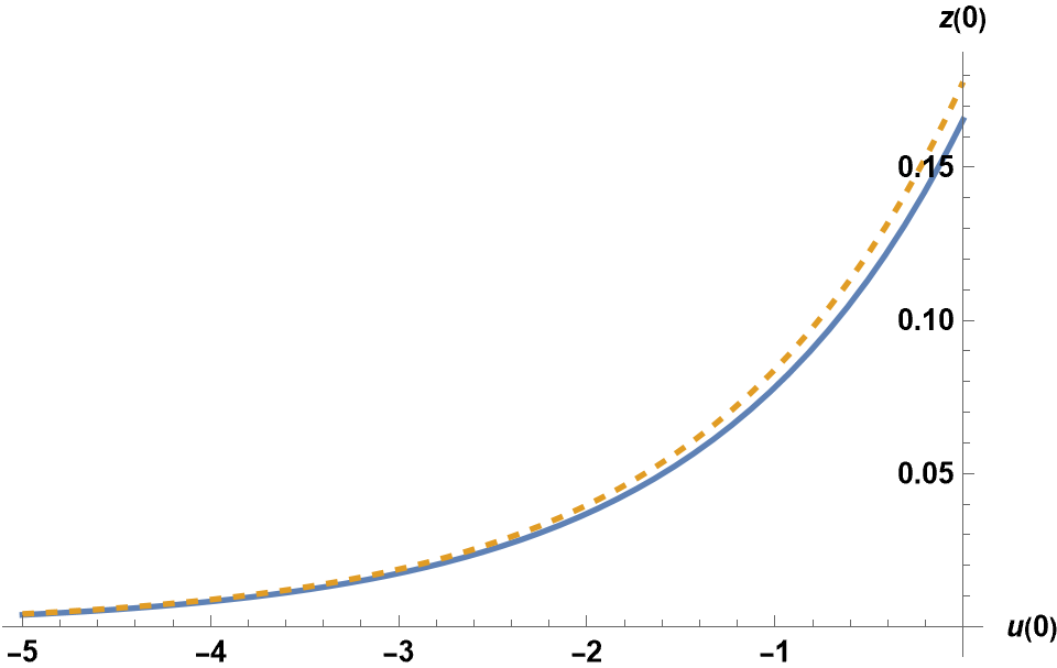
It is useful to know where (1 - 4 (1 - 1000 E^(-3 u[0]) z[0]^4)) vanishes:

up0 = Simplify[SolveValues[up^-2 == 0, z[0], Reals], u[0] \[Element] Reals] // Last
(* ((3/2)^(1/4) E^((3 u[0])/4))/(2 5^(3/4)) *)

Plot[{up0, zp0}, {u[0], -5, 0}, AxesLabel -> {u[0], z[0]}, 
    PlotStyle -> {Thick, Dashed}, LabelStyle -> {Bold, Black}]

enter image description here

Only values of {u[0], z[0]) above the solid curve yield real values for {u'[0], z'[0]). For completeness the dashed curve showing where z'[0] vanishes also is plotted.

zp0 = Simplify[SolveValues[zp[[2]] == 0, z[0], Reals], u[0] \[Element] Reals] // Last
(* ((3/2)^(1/4) E^((3 u[0])/4))/(2 5^(3/4)) *)

Now, search for solutions {u[x], z[x]} satisfying the desired {0.03, 0.01}.

f = ParametricNDSolveValue[{eq01, eq02, u[a] == u0, 
    z[a] == z0, {u'[a] == up, z'[a] == zp} /. {u[a] -> u0, z[a] -> z0}}, 
    Sqrt[(u[b] - .03)^2 + (z[b] - .01)^2], {x, a, b}, {u0, z0}];
ff[u1_, z1_] := If[1 - 4 (1 - 1000 Exp[-3 u1] z1^4) > 0, f[u1, z1], 1.]

FindMinimum[{ff[u1, z1], 1 - 4 (1 - 1000 Exp[-3 u1] z1^4) > 0}, {{u1, 0.}, {z1, .1769}}]
(* {0.153347, {u1 -> -0.075192, z1 -> 0.158538}} *)

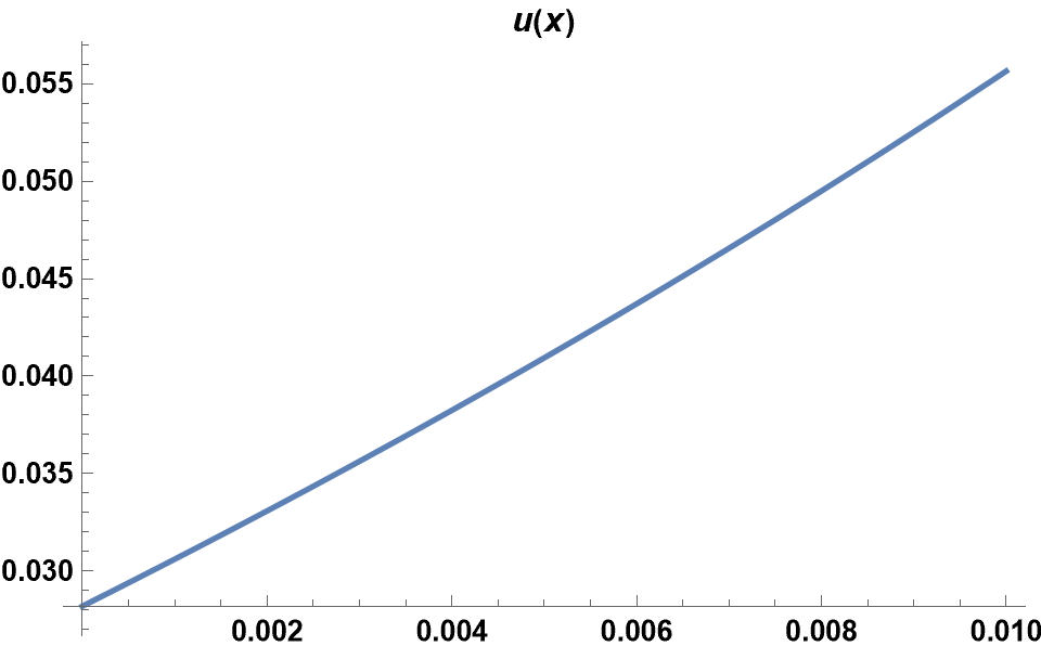
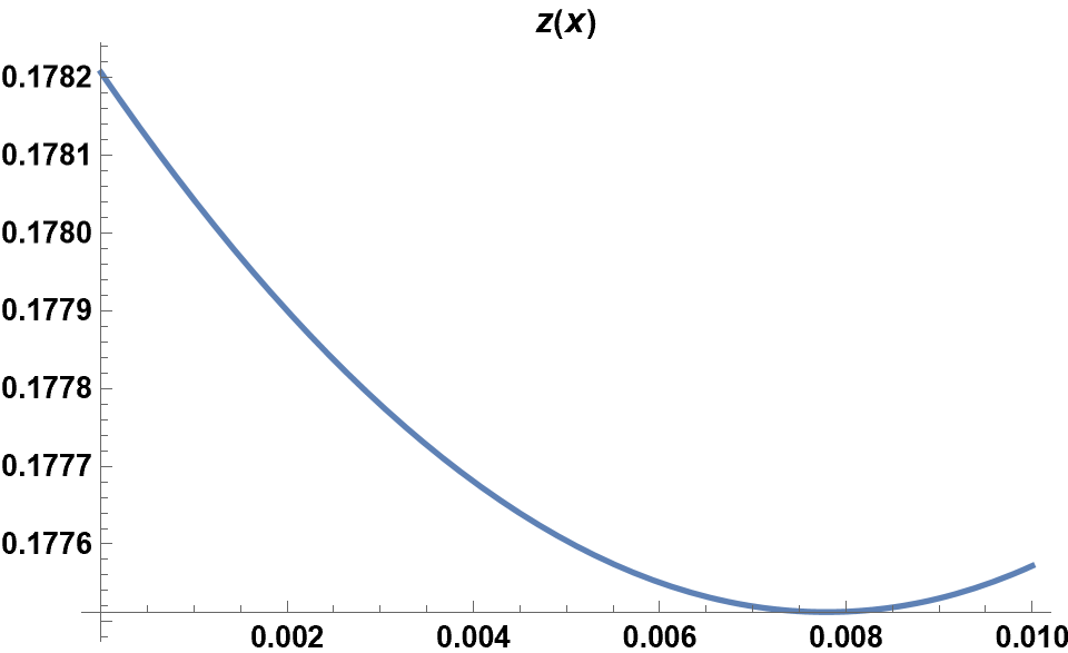
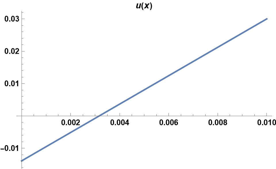
The residual is far too large for a valid solution.

ts = NDSolveValue[{eq01, eq02, u[a] == u1 /. Last[%], 
    z[a] == z1 /. Last[%], u'[a] == up, z'[a] == zp}, {u[x], z[x]}, {x, a, b}];
Plot[ts[[1]], {x, a, b}, PlotLabel -> u[x], LabelStyle -> {Bold, Black}]
Plot[ts[[2]], {x, a, b}, PlotLabel -> z[x], LabelStyle -> {Bold, Black}]

enter image description here enter image description here

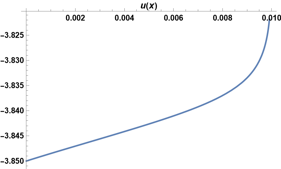
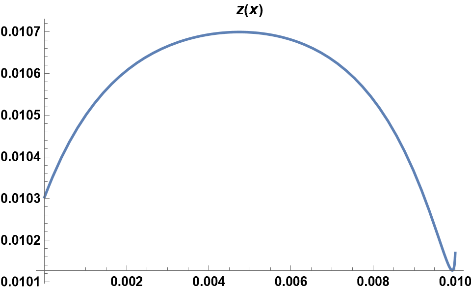
Because FindMinimum finds only a single local minimum, I tried several other starting values in the range -0.5 < u[0] < 0.5 with corresponding values of z[0] above the curve in the first plot. Results were comparable to the one just presented. For more negative values of u[0], FindMinimum (and also NMinimize) wandered into solution spaces where solutions grew explosively before reaching x = b. I did explore a few well-behaved solutions manually for u[0] in the vicinity of -4, but the resulting residuals were very large.

ts = NDSolveValue[{eq01, eq02, u[a] == -3.85, z[a] == .01030323, 
    u'[a] == up, z'[a] == zp}, {u[x], z[x]}, {x, a, b}];
Plot[ts[[1]], {x, a, b}, PlotLabel -> u[x], LabelStyle -> {Bold, Black}]
Plot[ts[[2]], {x, a, b}, PlotLabel -> z[x], LabelStyle -> {Bold, Black}]

enter image description here enter image description here

The analysis above does not prove that there are no solutions to this system of ODEs, but it certainly suggests it.

Equations (3) and (4) include leading signs that are either positive or negative. Choosing negative signs for both up and zp yields results similar to those above. When the leading sign was chosen negative for just one of up and zp, FindMinimum did not converge well. I did not explore this further.

Results based on code expressions in the question

The code in the question defines up and zp as

up = Sqrt[Sqrt[((d - 1)^2/(1 - (d - 1)^2 
    (1 - c Exp[-g u[0]] (z[0])^(d + 1))))^2]] /. d -> 3
zp = -(1 - c Exp[-g u[0]] (z[0])^(d + 1)) 
     Sqrt[Sqrt[((d - 1)^2/(1 - (d - 1)^2 
    (1 - c Exp[-g u[0]] (z[0])^(d + 1))))^2]] /. d -> 3
(* 2 (1/(1 - 4 (1 - 1000 E^(-3 u[0]) z[0]^4))^2)^(1/4) *)
(* 2 (-1 + 1000 E^(-3 u[0]) z[0]^4) 
     (1/(1 - 4 (1 - 1000 E^(-3 u[0]) z[0]^4))^2)^(1/4) *)

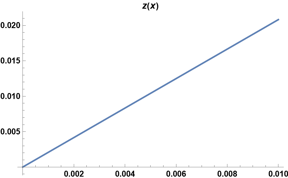
which gives real numbers everywhere except on the solid line in the first plot above. Then, with f defined as before (ff no longer is needed),

NMinimize[{f[u1, z1]}, {u1, z1}]
{0.0108168, {u1 -> -0.0139103, z1 -> 1.62312*10^-9}}

converges well. (FindMinimum yields similar results, although it does not converge as well.) Plotting the corresponding curves, as before, yields

enter image description here enter image description here

Incidentally, I attempted to reproduce as an initial value problem with NDSolve the last plots in the answer by Alex Trounev by using {u[0], u'[0], z[0], z'[0]} from his answer and comments, but the resulting curves did not resemble his plots. It is unclear why the results differ.

$\endgroup$
3
  • $\begingroup$ Please, see Update 2 to my answer. $\endgroup$ Commented Dec 9, 2023 at 15:50
  • $\begingroup$ Please, see Update 4 to my answer. :) $\endgroup$ Commented Dec 10, 2023 at 4:30
  • $\begingroup$ @bbgodfrey Very nice analysis and it helped me understand better the problem, definitely an upvote! Thanks! $\endgroup$
    – mathemania
    Commented Dec 13, 2023 at 15:27

Your Answer

By clicking “Post Your Answer”, you agree to our terms of service and acknowledge you have read our privacy policy.