Numerically finding a curve that satisfies an underdetermined set of equations

Question

I am trying to determine a phase diagram along the lines of Fig 3. or Fig 4. of this pubilcation. The curves plotted are binodals and are determined by the conditions of equality of chemical potentials of each component in all phases and equality of osmotic pressure in each phase (Section 4 of the SI is a good primer).

As an example, I use free energy function similar to the one defined in the paper (although the one I am actually interested in a bit more complex. Ideally I can come up with a solution that is robust and generally applicable). This is still a good starting point because my system does reduce to this under certain limits.

We narrow our attention to the case of two solutes (1 solvent) and 2 phases. Then we wish to find the locus of points in ($\phi_a,\phi_b$) for which the following conditions hold

$$\mu_a^{(1)} (\phi^{(1)}_a,\phi^{(1)}_b) = \mu_a^{(2)} (\phi^{(2)}_a,\phi^{(2)}_b)$$ $$\mu_b^{(1)} (\phi^{(1)}_a,\phi^{(1)}_b) = \mu_b^{(2)} (\phi^{(2)}_a,\phi^{(2)}_b)$$ $$\Pi^{(1)} (\phi^{(1)}_a,\phi^{(1)}_b) = \Pi^{(2)} (\phi^{(2)}_a,\phi^{(2)}_b)$$

Essentially, we have 4 unknowns $\phi^{(1)}_a,\phi^{(1)}_b, \phi^{(0)}_a,\phi^{(0)}_b$ and 3 equations. Subscripts here in my notation label the components and superscripts the phase. The solutions should look like the curves present in Fig 3 or Fig 4 of the linked publication (depending on parameter values). The conditions described above should be equivalent to equations (39)-(41) in this SI

Here are the function definitions

     F[a_, b_, uaa_, ubb_, uab_, na_, nb_] := 
     a/na*Log[a] + b/nb*Log[b] + (1 - a - b)*Log[1 - a - b + 10^-14] - 
      1/2*uaa*a^2 - 1/2*ubb*b^2 - uab*b*a 

    det[a_, b_, uaa_, ubb_, uab_, na_, nb_] := 
     Det[D[F[a, b, uaa, ubb, uab, na, nb], {{a, b}, 2}]] // Evaluate
    \[Mu]a[a_, b_, uaa_, ubb_, uab_, na_, nb_] := 
     D[F[a, b, uaa, ubb, uab, na, nb], a] // Evaluate
    \[Mu]b[a_, b_, uaa_, ubb_, uab_, na_, nb_] := 
     D[F[a, b, uaa, ubb, uab, na, nb], b] // Evaluate
   \[CapitalPi]F[a_, b_, uaa_, ubb_, uab_, na_, 
  nb_] := \[Mu]a[a, b, uaa, ubb, uab, na, nb]*
    a + \[Mu]b[a, b, uaa, ubb, uab, na, nb]*b - 
   F[a, b, uaa, ubb, uab, na, nb] // Evaluate

My first thought was to use NSolve

    NSolve[{\[Mu]a[a1, b1, 0, 0, 4.36, 10, 6] == \[Mu]a[a2, b2, 0, 0, 
    4.36, 10, 6],
  \[Mu]b[a1, b1, 0, 0, 4.36, 10, 6] == \[Mu]b[a2, b2, 0, 0, 4.36, 10, 
    6],
  \[CapitalPi]F[a1, b1, 0, 0, 4.36, 10, 6] == \[CapitalPi]F[a2, b2, 0,
     0, 4.36, 10, 6], a1 >= 0, b1 >= 0, a2 >= 0, b2 >= 0, 
  a2 + b2 <= 1, a1 + b1 <= 1
  }, {a1, b1, a2, b2}, Reals]

but it seems like that is not the right way to do it.

Alternatively, I thought of using FindRoot combined with grid search in the region, but I am not quite sure how to implement it, or if it is the optimum most efficient way to solve this problem. An intelligent way of choosing seed values for FindRoot might be to use the spinodal which can be visualized as follows. Since if I understand correctly the binodal curve we are interested in should envelop this so we can try seeding points on the exterior of this?

Manipulate[ContourPlot[det[a, b, uaa, ubb, uab, 10, 6] == 0,
  {a, 0, 1}, {b, 0, 1}],
 {uaa, 0, 10}, {uab, 0, 10}, {ubb, 0, 10}]

Q1 : Is there any other built-in function in mathematica that can help me solve my problem? Q2 : If not are there any standard approaches/algorithms that can be applied to this situation ?

EDIT : Partially Cross-posted Stack Overflow. Includes a janky-python brute force solution attempt using a grid search I attempted.

Answer 1

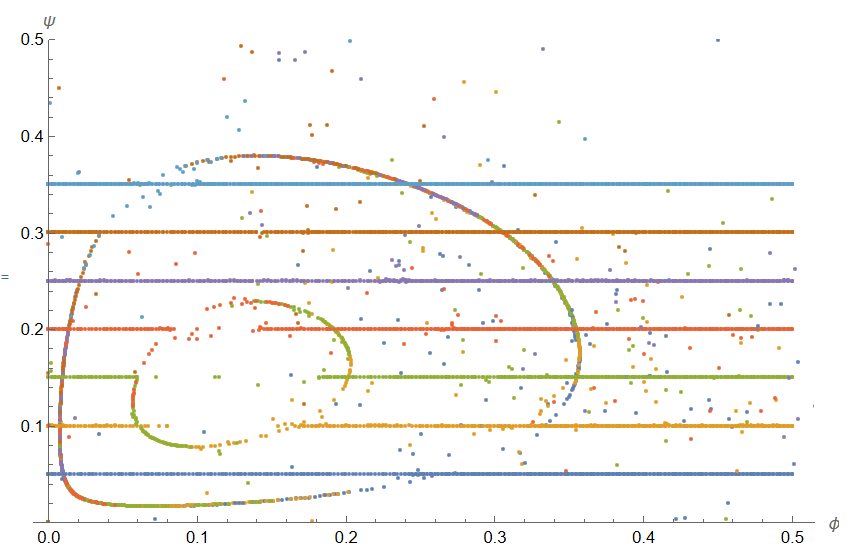
We can compute data shown in Figure 4 from the paper cited using NMinimize and expression for the free energy as follows

lst = Join[{{0, 0}}, 
  Table[{x, x Log[x]}, {x, 10^-3, 1, 10^-3}]]; xlog = 
 Interpolation[lst];

F[a_, b_] := 
  Module[{uaa = 0, ubb = 0, uab = 4.36, na = 10, nb = 6, F, mua, mub, 
    PiF, det}, 
   1/na*xlog[a] + 1/nb*xlog[b] + xlog[1 - a - b] - 1/2*uaa*a^2 - 
    1/2*ubb*b^2 - uab*b*a];


freeE[x_, a1_, b1_, a2_, b2_, p1_, 
   p2_] := {x F[a1, b1] + (1 - x) F[a2, b2], {x >= 0, x <= 1, a1 >= 0,
     a2 >= 0, b1 >= 0, b2 >= 0, a1 <= 1, b1 <= 1, a2 <= 1, b2 <= 1, 
    x a1 + (1 - x) a2 == p1, x b1 + (1 - x) b2 == p2}};

r = Range[0, .5, .0025]; Do[p2 = .05 i; 
 ls[i] = Table[{a1, b1, a2, b2, x} /. 
     NMinimize[
       freeE[x, a1, b1, a2, b2, p1, p2], {a1, b1, a2, b2, x}][[2]] // 
    Quiet, {p1, r}];, {i, 7}];

Visualization

Show[ListPlot[
  Table[Transpose[{ls[i][[All, 1]], ls[i][[All, 2]]}], {i, 7}], 
  PlotRange -> All, AxesLabel -> {"\[Phi]", "\[Psi]"}], 
 ListPlot[
  Table[Transpose[{ls[i][[All, 3]], ls[i][[All, 4]]}], {i, 7}], 
  PlotRange -> All]]

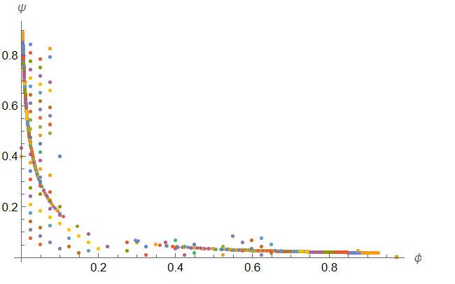
Same picture we compute at uab = 3.8 and combine two pictures as

Update 1. To compute data shown in Figure 3 we use code

lst = Join[{{0, 0}}, 
  Table[{x, x Log[x]}, {x, 10^-3, 1, 10^-3}]]; xlog = 
 Interpolation[lst];

F[a_, b_] := 
  Module[{uaa = 1.8, ubb = 0, uab = 0, na = 10, nb = 6, F, mua, mub, 
    PiF, det}, 
   1/na*xlog[a] + 1/nb*xlog[b] + xlog[1 - a - b] - 1/2*uaa*a^2 - 
    1/2*ubb*b^2 - uab*b*a];


freeE[x_, a1_, b1_, a2_, b2_, p1_, 
   p2_] := {x F[a1, b1] + (1 - x) F[a2, b2], {x >= 0, x <= 1, a1 >= 0,
     a2 >= 0, b1 >= 0, b2 >= 0, a1 <= 1, b1 <= 1, a2 <= 1, b2 <= 1, 
    x a1 + (1 - x) a2 == p1, x b1 + (1 - x) b2 == p2}};

r = Range[0, 1, .0125]; Do[p2 = If[.1 i - p1 > 0, .1 i - p1, 0]; 
 ls[i] = Table[{a1, b1, a2, b2, x} /. 
     NMinimize[
       freeE[x, a1, b1, a2, b2, p1, p2], {a1, b1, a2, b2, x}][[2]] // 
    Quiet, {p1, r}];, {i, 0, 10, 1}];

Visualization

Show[ListPlot[
  Table[Transpose[{ls[i][[All, 1]], ls[i][[All, 2]]}], {i, 0, 10, 1}],
   PlotRange -> All, AxesLabel -> {"\[Phi]", "\[Psi]"}], 
 ListPlot[
  Table[Transpose[{ls[i][[All, 3]], ls[i][[All, 4]]}], {i, 0, 10, 1}],
   PlotRange -> All]]

And the same picture we compute for uaa = 1.3, finally we have

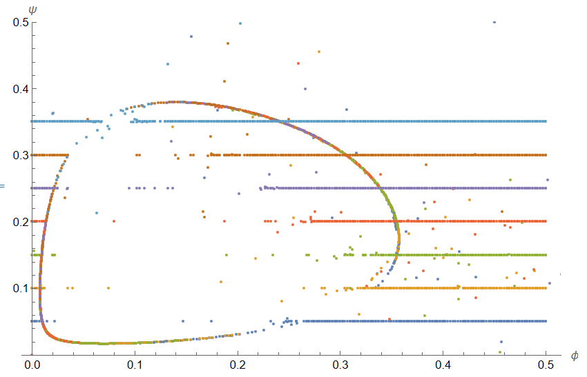
Update 2. We can use equations for $\mu_a, \mu_b, \Pi$ as a filter for solutions computed above as follows

lst = Join[{{0, 0}}, 
  Table[{x, x Log[x]}, {x, 10^-3, 1, 10^-3}]]; xlog = 
 Interpolation[lst];

fun = Module[{uaa = 1.3, ubb = 0, uab = 0, na = 10, nb = 6, F, mua, 
    mub, PiF, det}, 
   F = a/na*Log[a] + b/nb*Log[b] + (1 - a - b)*Log[1 - a - b] - 
     1/2*uaa*a^2 - 1/2*ubb*b^2 - uab*b*a;
   det = Det[D[F, {{a, b}, 2}]];
   mua = D[F, a];
   mub = D[F, b];
   PiF = mua*a + mub*b - F; {mua, mub, PiF, det, F}];

F[a_, b_] := 
  Module[{uaa = 1.3, ubb = 0, uab = 0, na = 10, nb = 6, F, mua, mub, 
    PiF, det}, 
   1/na*xlog[a] + 1/nb*xlog[b] + xlog[1 - a - b] - 1/2*uaa*a^2 - 
    1/2*ubb*b^2 - uab*b*a];


freeE[x_, a1_, b1_, a2_, b2_, p1_, 
   p2_] := {x F[a1, b1] + (1 - x) F[a2, b2], {x >= 0, x <= 1, a1 >= 0,
     a2 >= 0, b1 >= 0, b2 >= 0, a1 <= 1, b1 <= 1, a2 <= 1, b2 <= 1, 
    x a1 + (1 - x) a2 == p1, x b1 + (1 - x) b2 == p2}};

r = Range[0, 1, 1/40]; r1 = Range[0, 9/10, 1/30]; Do[
 p2 = If[i - p1 > 0, i - p1, 0]; 
 sol[i, p1] = 
  NMinimize[freeE[x, a1, b1, a2, b2, p1, p2], {a1, b1, a2, b2, x}][[
    2]] // Quiet;, {p1, r}, {i, r1}];

eqmua1 = fun[[1]] /. {a -> a1, b -> b1}; eqmua2 = 
 fun[[1]] /. {a -> a2, b -> b2};

eqmua = eqmua1 - eqmua2 // Simplify;

eqmub1 = fun[[2]] /. {a -> a1, b -> b1}; eqmub2 = 
 fun[[2]] /. {a -> a2, b -> b2};

eqmub = eqmub1 - eqmub2 // Simplify;
eqpi1 = fun[[3]] /. {a -> a1, b -> b1}; eqpi2 = 
 fun[[3]] /. {a -> a2, b -> b2};

eqpi = eqpi1 - eqpi2 // Simplify

Do[ls[i] = 
    Table[If[(Norm[{eqmua, eqmub, eqpi}] /. sol[i, p1] /. 
         Indeterminate -> 1) <= 10^-3, {a1, b1, a2, b2, x} /. 
       sol[i, p1], Nothing], {p1, r}];, {i, r1}];  

Visualization

Show[ListPlot[
  Table[Transpose[{ls[i][[All, 1]], ls[i][[All, 2]]}], {i, r1}], 
  PlotRange -> All, AxesLabel -> {"\[Phi]", "\[Psi]"}], 
 ListPlot[
  Table[Transpose[{ls[i][[All, 3]], ls[i][[All, 4]]}], {i, r1}], 
  PlotRange -> All]]