49
$\begingroup$

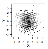
Hexagon bin plots are a useful way of visualising large datasets of bivariate data. Here are a few examples:

With bin frequency indicated by grey level...

enter image description here

..and by glyph size

enter image description here

There are packages for creating this kind of plot in both "R" and Python. Obviously, the idea is similar to DensityHistogram plots.

How would one go about generating hexagonal bins in Mathematica? Also, how would one control the size of a plotmarker based on the bin frequency?

Update

As a starting point I have tried to create a triangular grid of points:

vert1 = Table[{x, Sqrt[3] y}, {x, 0, 20}, {y, 0, 10}];
vert2 = Table[{1/2 x, Sqrt[3] /2 y}, {x, 1, 41, 2}, {y, 1, 21, 2}];

verttri = Flatten[Join[vert1, vert2], 1];

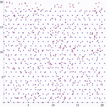
overlaying some data..

data = RandomReal[{0, 20}, {500, 2}];

ListPlot[{verttri, data}, AspectRatio -> 1]

enter image description here

next step might involve using Nearest:

nearbin = Nearest[verttri];

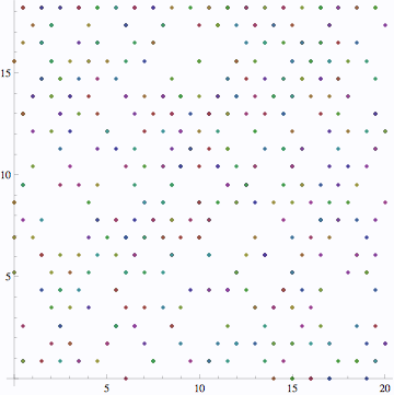
ListPlot[nearbin[#] & /@ data, AspectRatio -> 1]

enter image description here

This gives the location of vertices with nearby data points. Unfortunately, I can't see how to count those data points..

$\endgroup$
5
  • $\begingroup$ Do you know about SmoothDensityHistogram - and likewise DensityHistogram? $\endgroup$
    – Jens
    Commented Jul 6, 2013 at 5:38
  • $\begingroup$ MMA's VoronoiDiagram will be too slow for your needs. $\endgroup$
    – VF1
    Commented Jul 6, 2013 at 5:49
  • $\begingroup$ @Jens, Yes I am aware of these functions. Not quite what I am looking for. Depending on the context I think hexagonal binning gives better representation of the data due to it's regular tessellated symmetry and nearest neighbour optimisation than a square grid. $\endgroup$
    – geordie
    Commented Jul 6, 2013 at 6:01
  • 2
    $\begingroup$ @geordie OK - so you insist on hexbins. That means work. The bins form a honeycomb lattice, which is not the same as a hexagonal lattice because it's not a 2D Bravias lattice. You have to choose two Bravais lattice basis vectors and two more basis vectors for the unit cell. Then for each data point, project its coordinate on those vectors, find the integer part of the projections and count them. That will lead to the histogram count for each cell. It doesn't involve finding Voronoi diagrams or using Nearest (too slow). Don't have time to execute these steps myself... $\endgroup$
    – Jens
    Commented Jul 6, 2013 at 6:10
  • $\begingroup$ @Jens. Yes, the question is about hexagon bin plots. What you are suggesting sounds interesting. It's a pity you don't have the time to elaborate... $\endgroup$
    – geordie
    Commented Jul 6, 2013 at 6:33

3 Answers 3

29
$\begingroup$

With the set-up you already have, you can do

nearbin = Nearest[Table[verttri[[i]] -> i, {i, Length@verttri}]];
counts = BinCounts[nearbin /@ data, {1, Length@verttri + 1, 1}];

which counts the number of data points nearest to each vertex. Then just draw the glyphs directly:

With[{maxCount = Max@counts}, 
 Graphics[
  Table[Disk[verttri[[i]], 0.5 Sqrt[counts[[i]]/maxCount]], {i, Length@verttri}],
  Axes -> True]]

The square root is so that the area of the glyphs, and the number of black pixels, corresponds to the number of data points in each bin. I used data = RandomVariate[MultinormalDistribution[{10, 10}, 7 IdentityMatrix[2]], 500] to get the following plot:
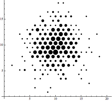
enter image description here

As Jens has commented already, though, this is a unnecessarily slow way of going about it. One ought to be able to directly compute the bin index from the coordinates of a data point without going through Nearest. This way was easy to implement and works fine for a 500-point dataset though.


Update: Here's an approach that doesn't require you to set up a background grid in advance. We'll directly find the nearest grid vertex for each data point and then tally them up. To do so, we'll break the hexagonal grid into rectangular tiles of size $1\times\sqrt3$. As it turns out, when you're in say the $[0,1]\times[0,\sqrt3]$ tile, your nearest grid vertex can only be one of the five vertices in the tile, $(0,0)$, $(1,0)$, $(1/2,\sqrt3/2)$, $(0,\sqrt3)$, and $(1,\sqrt3)$. We could work out the conditions explicitly, but let's just let Nearest do the work:

tileContaining[{x_, y_}] := {Floor[x], Sqrt[3] Floor[y/Sqrt[3]]};
nearestWithinTile = Nearest[{{0, 0}, {1, 0}, {1/2, Sqrt[3]/2}, {0, Sqrt[3]}, {1, Sqrt[3]}}];
nearest[point_] := Module[{tile, relative},
   tile = tileContaining[point];
   relative = point - tile;
   tile + First@nearestWithinTile[relative]];

The point is that a NearestFunction over just five points ought to be extremely cheap to evaluate—certainly much cheaper than your NearestFunction over the several hundred points in verttri. Then we just have to apply nearest on all the data points and tally the results.

tally = Tally[nearest /@ data];
With[{maxTally = Max[Last /@ tally]}, 
 Graphics[
  Disk[#[[1]], 1/2 Sqrt[#[[2]]/maxTally]] & /@ tally, 
  Axes -> True, AxesOrigin -> {0, 0}]]
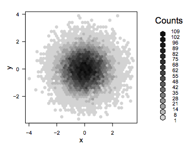
$\endgroup$
1
  • 1
    $\begingroup$ Nice update. This is indeed a lot faster. $\endgroup$
    – geordie
    Commented Jul 7, 2013 at 7:37
26
$\begingroup$

As this answer got much more attention than I thought at first, I felt compelled to pack the answer as a function.

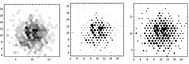
The following function draws three different hex-histogram representations of your data.

Code stolen liberally from the question and from Rahul's answer.

f[data_, cs_, ptype_] :=
 Module[{hc, vh, nearbin, counts, trr, maxCount},
  hc = Flatten[Table[{i, j}, (*hexagons positions*)
     {p, 0, 1},
     {j, 3 p/2 cs + Min[data[[All, 2]]], Max[data[[All, 2]]], 3 cs},
     {i, p Sqrt[3]/2 cs + Min[data[[All, 1]]], Max[data[[All, 1]]], 
      Sqrt[3] cs}], 2];

  vh = cs Vertices[Hexagon];
  nearbin = Nearest[Table[hc[[i]] -> i, {i, Length@hc}]];
  counts = BinCounts[nearbin /@ data, {1, Length@hc + 1, 1}];
  trr[v_, tr_] := Translate[Rotate[Polygon[v], Pi/2], tr];
  maxCount = Max@counts;

  Graphics[Table[
    Switch[ptype,
     1, {Opacity[counts[[n]]/maxCount], trr[vh, hc[[n]]]},
     2, trr[counts[[n]]/maxCount vh, hc[[n]]],
     3, trr[Sqrt[counts[[n]]/maxCount] vh, hc[[n]]]],
    {n, Length@hc}],
   Axes -> True]
  ]

<< Polytopes`
cs = 1/2;(*cell size*)
data = RandomVariate[MultinormalDistribution[{10, 10}, 7 IdentityMatrix[2]], 500];
GraphicsRow@Table[f[data, cs, i], {i, 3}]

Mathematica graphics

The old answer can be found in the post's edit history - removed

$\endgroup$
10
  • $\begingroup$ This is great. I have incorporated your answer into a standalone function with inputs honeybin[xdata_, ydata_, cs_, {{xmin_, xmax_}, {ymin_, ymax_}}]:=... and the dimensions of the verttri array set by Max@xdata + padding etc. I can post it as an answer unless you want to do something similar? Also, I couldn't find a way to crop the hexagons within the axes (i also tried Framed->True). any suggestions? should I post what I have? $\endgroup$
    – geordie
    Commented Jul 7, 2013 at 4:15
  • 2
    $\begingroup$ +1 that's sweet (like honey! :)). You can do it without the Polytopes package: Hexagon[w_] := Polygon[w + N[#] & /@ (Through[{Cos, Sin}[Pi # /3]] & /@ Range[0, 6])]; then ..Rotate[Hexagon[cs] ... $\endgroup$
    – cormullion
    Commented Jul 7, 2013 at 6:54
  • 1
    $\begingroup$ @geordie Re: Cropping. Try with these two options combined: PlotRange -> { {...},{...} } and PlotRangeClipping -> True $\endgroup$ Commented Jul 7, 2013 at 13:35
  • 1
    $\begingroup$ @geordie I tried to make a standalone function. See if it fits you $\endgroup$ Commented Jul 7, 2013 at 14:34
  • $\begingroup$ You may want to steal from my updated answer, too... :) $\endgroup$
    – user484
    Commented Jul 7, 2013 at 16:29
17
$\begingroup$

Here is a standalone function incorporating belisarius' standalone framework and Rahul Narain's fast use of NearestFunction. Full credit to these guys!

 Needs["Polytopes`"];
 honeybin[data_, cs_, ptype_, {{xmin_, xmax_}, {ymin_, ymax_}}] :=

 (*"cs_" is the width of a bin,i.e.the distance between bin centers*)

  Module[{tileContaining, nearestWithinTile, nearest, tally, vh, hexr,
    trr},

   tileContaining[{x_, y_}] := {Floor[x], Sqrt[3] Floor[y/Sqrt[3]]};
   nearestWithinTile = 
     Nearest[{{0, 0}, {1, 0}, {1/2, Sqrt[3]/2}, {0, Sqrt[3]}, {1, Sqrt[3]}}];
   nearest[point_] := Module[{tile, relative}, tile = tileContaining[point];
   relative = point - tile;
     tile + First@nearestWithinTile[relative]];

   vh = cs 1.05 Vertices[Hexagon]/Sqrt[3];
   trr[v_, tr_] := Translate[Rotate[Polygon[v], Pi/2], tr];
   tally = Tally[cs (nearest /@ (data/cs))];

  With[{maxTally = Max[Last /@ tally]},  
   Graphics[Table[
     Switch[ptype,
      1, {Blend[{Lighter[Red, 0.99], Darker[Red, 0.6]},
         Sqrt[Last@tally[[n]]/maxTally]], trr[vh, First@tally[[n]]]},
      2, trr[Last@tally[[n]]/maxTally vh, First@tally[[n]]], 
      3, trr[Sqrt[Last@tally[[n]]/maxTally] vh, First@tally[[n]]]], 
         {n, Length@tally}], 
    Frame -> True, 
    PlotRange -> {{xmin, xmax}, {ymin, ymax}}, 
    PlotRangeClipping -> True]]]

note there is a fudge factor (1.05) to get rid of whitespace between the cells.

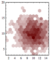
With a little Colour...

data = RandomVariate[MultinormalDistribution[{10, 10}, 7 IdentityMatrix[2]], 1000];
honeybin[data, 1, 1, {{1, 15}, {3, 20}}]

enter image description here

$\endgroup$
8
  • 1
    $\begingroup$ Nice! By the way, the easiest way to do a different bin size is to divide all the data by cs, bin them, and then multiply the bin positions by cs. $\endgroup$
    – user484
    Commented Jul 8, 2013 at 4:55
  • 1
    $\begingroup$ There, I fixed it. I changed the meaning of cs to "the width of a cell" so the original cells in the question correspond to cs = 1. Also, the results were no longer up to date, so I removed them; sorry if you're not happy about that. $\endgroup$
    – user484
    Commented Jul 8, 2013 at 16:29
  • 1
    $\begingroup$ By the way, your function doesn't work for me unless I take << Polytopes`; out of the function, but I don't know if that's me doing something wrong or what, so I haven't touched it. $\endgroup$
    – user484
    Commented Jul 8, 2013 at 16:30
  • 2
    $\begingroup$ Geordie: ClearAll["Global`"] only clears variables in the Global context, whereas your package definitions live inside its context. It is certainly possible to load a package in a function and use it immediately. With your previous definition, when you evaluate that cell, the symbols Vertices and Hexagon are created in the Global context at the parsing stage, but they're supposed to be in the Polytopes context. You could instead define them with their long forms as Polytopes`Vertices so that it is created in that context at parse time. You'll get a shadowing warning otherwise @Rah $\endgroup$
    – rm -rf
    Commented Jul 9, 2013 at 0:43
  • 1
    $\begingroup$ polytopes is unnecessary if Vertices[Hexagon] is replaced by CirclePoints[6] in version 13. Thanks for the code. The speed up starts to work at 2000 points. $\endgroup$
    – NigelKg
    Commented Aug 10, 2022 at 10:47

Your Answer

By clicking “Post Your Answer”, you agree to our terms of service and acknowledge you have read our privacy policy.

Not the answer you're looking for? Browse other questions tagged or ask your own question.