Parting a table by second column elements

Question

I have 2 X m table with elements {{x1, y1}, {x2, y2}, .... {xi, yi}, .....{xm, ym}}. It is an experimental data, which can be seen in the attached picture. There is a significant noise and arbitrariness in the variation of independent parameter (first column, x) as well as dependent double valued parameter (second column, y). Here, I want to divide the data into two parts- one which has almost constant y and another with y increasing with x. How to achieve it as the inflection point may not be in the center of the table.

Will appreciate any suggestion. Thanks
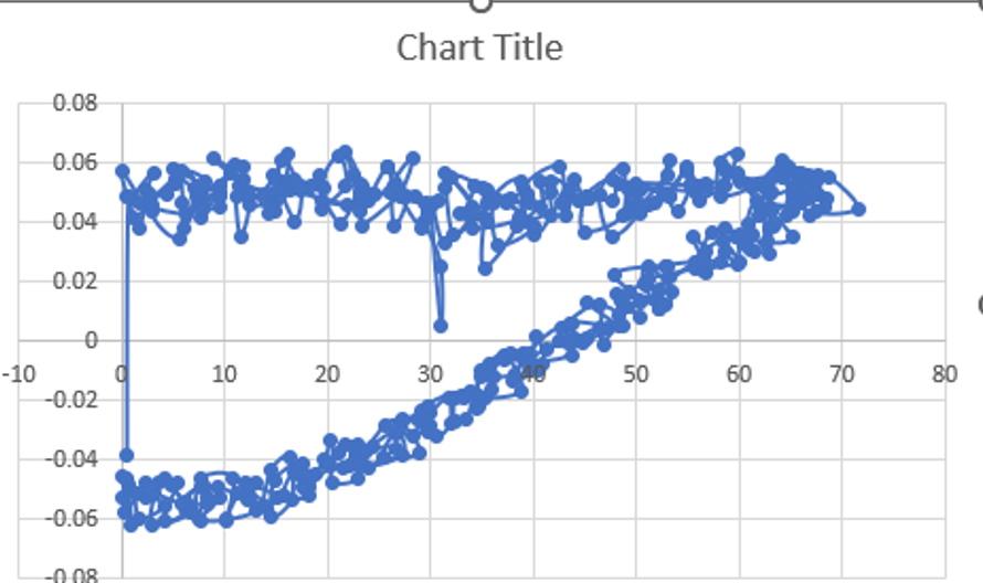
Here is a sample data -

{{40.3595,0.001477},{40.9698,-0.007586},{38.0707,-0.013534},{39.5966,-0.003783},{42.6483,0.004349},{43.869,-0.00443},{39.7491,-0.006777},{42.4957,-0.00002},{43.7164,0.001113},{41.3513,-0.002448},{43.9453,0.000263},{46.463,0.004875},{44.7845,-0.000506},{43.4113,-0.000182},{43.7164,0.00617},{47.3022,0.004268},{45.2423,0.000829},{43.4875,0.005887},{46.3867,0.012643},{46.6156,0.003864},{46.7682,-0.001153},{48.2941,0.008921},{45.2423,0.013008},{48.2178,0.00532},{48.6755,0.004956},{48.0652,0.015718},{49.1333,0.011996},{50.4303,0.008152},{48.5992,0.013534},{50.8881,0.019198},{52.0325,0.014343},{50.4303,0.013088},{49.3622,0.016487},{52.7954,0.012117},{52.1851,0.010863},{50.7355,0.019683},{51.1169,0.025428},{53.4821,0.016649},{52.2614,0.011268},{47.9126,0.022273},{52.8717,0.025186},{53.1769,0.021828},{52.2614,0.017782},{55.6946,0.02644},{55.6946,0.024457},{51.1169,0.021221},{53.0243,0.025469},{58.2886,0.026804},{56.6864,0.023486},{56.6101,0.026683},{55.4657,0.035098},{56.839,0.030324},{56.6101,0.02381},{56.4575,0.028908},{58.3649,0.033561},{59.8145,0.026238},{56.4575,0.026521},{57.373,0.036797},{59.6619,0.035584},{59.967,0.02648},{58.5938,0.030203},{58.5175,0.037971},{60.3485,0.034896},{61.4929,0.030364},{60.0433,0.035705},{61.3403,0.035988},{61.1877,0.031052},{60.73,0.032671},{61.9507,0.0423},{62.8662,0.038254},{62.9425,0.029474},{60.9589,0.039508},{61.9507,0.046305},{65.155,0.034977},{62.7136,0.033803},{62.9425,0.045294},{65.155,0.043837},{63.4003,0.039063},{63.2477,0.043797},{68.4357,0.048166},{66.6046,0.048247},{64.621,0.042583},{65.155,0.049663},{67.5964,0.049299},{66.0706,0.046629},{66.2231,0.049097},{67.3676,0.05379},{68.2068,0.045456},{66.7572,0.042259},{65.5365,0.056541},{68.8171,0.054963},{71.5637,0.044646},{67.5201,0.043716},{67.5964,0.055773},{66.6809,0.056056},{67.5201,0.049299},{67.4438,0.049501},{66.7572,0.054437},{65.918,0.052981},{67.4438,0.053669},{66.2231,0.056218},{67.3676,0.050634},{65.4602,0.048288},{64.4684,0.055732},{66.0706,0.056541},{67.2913,0.049259},{65.3839,0.046629},{64.6973,0.059171},{64.0869,0.061315},{65.4602,0.052415},{62.8662,0.049501},{63.9343,0.058483},{63.5529,0.056703},{63.1714,0.050634},{61.4166,0.052779},{64.1632,0.055611},{63.2477,0.055449},{60.1196,0.054073},{58.8989,0.056825},{62.561,0.05205},{61.7218,0.0476},{59.8145,0.056784},{58.67,0.058079},{61.1115,0.052172},{58.2123,0.049097},{58.136,0.060304},{59.8907,0.063338},{58.5175,0.052576},{56.1523,0.0476},{56.6864,0.053062},{58.3649,0.052698},{55.6946,0.050351},{48.2941,0.053264},{55.2368,0.052415},{56.839,0.051848},{55.9998,0.052293},{55.0079,0.057148},{53.1769,0.049056},{54.1687,0.043999},{55.3894,0.053264},{54.8553,0.058888},{53.3295,0.048935},{50.2777,0.043999},{53.1006,0.056096},{53.2532,0.061032},{51.8799,0.046912},{49.8199,0.046184},{50.4303,0.050837},{52.5665,0.049259},{51.1169,0.046346},{49.1333,0.051929},{50.6592,0.045172},{49.1333,0.043069},{49.5911,0.051363},{50.0488,0.053264},{50.2777,0.04323},{47.6074,0.035341},{46.463,0.049866},{48.6755,0.058322},{48.6755,0.042098},{44.9371,0.037},{45.166,0.048773},{47.76,0.054802},{47.76,0.0476},{45.2423,0.048571},{44.3268,0.047155},{45.4712,0.048207},{44.8608,0.047843},{44.0216,0.054559},{43.1824,0.048652},{43.2587,0.042219},{43.6401,0.050756},{41.6565,0.054235},{41.7328,0.042502},{39.978,0.035867},{39.1388,0.051524},{42.4957,0.058928},{42.7246,0.046508},{39.444,0.040479},{41.6565,0.050027},{40.741,0.053628}}

Answer 1

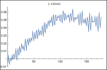
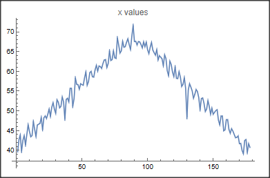
Store your data in d. Then we plot the x and y values separately:

ListLinePlot[d[[All, 2]], PlotLabel -> "y values"]

ListLinePlot[d[[All, 1]], PlotLabel -> "x values"]

You can see that the x and y values increase up to index 89. From there the x values decrease again, but the y values stay approx. constant.

The division of the data into two sets: d1 and d2 is therefore simple, take the first 89 points and the rest:

d1= Take[d,;;89];
d2= Take[d,90;;];

Answer 2

I am going to use QRMon because the workflow is easier to specify.

Procedure

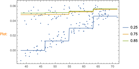
1. Fit Quantile Regression (QR) curves:

   1. Using small number of knots

   2. At different probabilities (e.g. 0.25 and 0.75)

   3. With different, low interpolation orders (e.g. 0, 1, 2)

2. Select QR parameters to extract the "near constant y" points.

3. Pick the points around produced regression quantile.

   1. Using suitable pick range (e.g. 0.015)

4. Plot the original data points and the extracted ones.

Code

Import["https://raw.githubusercontent.com/antononcube/MathematicaForPrediction/master/MonadicProgramming/MonadicQuantileRegression.m"]

qrObj = 
   QRMonUnit[data]⟹
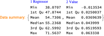
    QRMonEchoDataSummary⟹
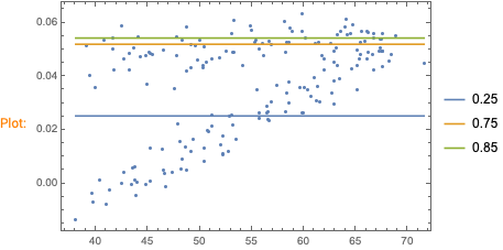
    QRMonQuantileRegression[4, {0.25, 0.75, 0.85}, InterpolationOrder -> 0]⟹
    QRMonPlot[];

qrObj = 
   QRMonUnit[data]⟹
    QRMonQuantileRegression[1, {0.25, 0.75, 0.85}, InterpolationOrder -> 0]⟹
    QRMonPlot[]⟹
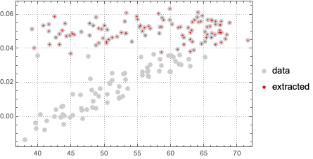
    QRMonPickPathPoints[0.015];

lsConstantYPoints = (qrObj⟹QRMonTakeValue)[0.75]

(*{{58.5175, 0.037971}, {61.9507, 0.0423}, {62.8662, 0.038254}, {60.9589, 0.039508}, {61.9507, 0.046305}, {62.9425, 0.045294}, {65.155, 0.043837}, {63.4003, 0.039063}, {63.2477, 0.043797}, {68.4357, 0.048166}, {66.6046, 0.048247}, {64.621, 0.042583}, {65.155, 0.049663}, {67.5964, 0.049299}, {66.0706, 0.046629}, {66.2231, 0.049097}, {67.3676, 0.05379}, {68.2068, 0.045456}, {66.7572, 0.042259}, {65.5365, 0.056541}, {68.8171, 0.054963}, {71.5637, 0.044646}, {67.5201, 0.043716}, {67.5964, 0.055773}, {66.6809, 0.056056}, {67.5201, 0.049299}, {67.4438, 0.049501}, {66.7572, 0.054437}, {65.918, 0.052981}, {67.4438, 0.053669}, {66.2231, 0.056218}, {67.3676, 0.050634}, {65.4602, 0.048288}, {64.4684, 0.055732}, {66.0706, 0.056541}, {67.2913, 0.049259}, {65.3839, 0.046629}, {64.6973, 0.059171}, {64.0869, 0.061315}, {65.4602, 0.052415}, {62.8662, 0.049501}, {63.9343, 0.058483}, {63.5529, 0.056703}, {63.1714, 0.050634}, {61.4166, 0.052779}, {64.1632, 0.055611}, {63.2477, 0.055449}, {60.1196, 0.054073}, {58.8989, 0.056825}, {62.561, 0.05205}, {61.7218, 0.0476}, {59.8145, 0.056784}, {58.67, 0.058079}, {61.1115, 0.052172}, {58.2123, 0.049097}, {58.136, 0.060304}, {59.8907, 0.063338}, {58.5175, 0.052576}, {56.1523, 0.0476}, {56.6864, 0.053062}, {58.3649, 0.052698}, {55.6946, 0.050351}, {48.2941, 0.053264}, {55.2368, 0.052415}, {56.839, 0.051848}, {55.9998, 0.052293}, {55.0079, 0.057148}, {53.1769, 0.049056}, {54.1687, 0.043999}, {55.3894, 0.053264}, {54.8553, 0.058888}, {53.3295, 0.048935}, {50.2777, 0.043999}, {53.1006, 0.056096}, {53.2532, 0.061032}, {51.8799, 0.046912}, {49.8199, 0.046184}, {50.4303, 0.050837}, {52.5665, 0.049259}, {51.1169, 0.046346}, {49.1333, 0.051929}, {50.6592, 0.045172}, {49.1333, 0.043069}, {49.5911, 0.051363}, {50.0488, 0.053264}, {50.2777, 0.04323}, {46.463, 0.049866}, {48.6755, 0.058322}, {48.6755, 0.042098}, {44.9371, 0.037}, {45.166, 0.048773}, {47.76, 0.054802}, {47.76, 0.0476}, {45.2423, 0.048571}, {44.3268, 0.047155}, {45.4712, 0.048207}, {44.8608, 0.047843}, {44.0216, 0.054559}, {43.1824, 0.048652}, {43.2587, 0.042219}, {43.6401, 0.050756}, {41.6565, 0.054235}, {41.7328, 0.042502}, {39.1388, 0.051524}, {42.4957, 0.058928}, {42.7246, 0.046508}, {39.444, 0.040479}, {41.6565, 0.050027}, {40.741, 0.053628}}*)

ListPlot[{data, lsConstantYPoints}, PlotTheme -> "Detailed", PlotStyle -> {{GrayLevel[0.8], PointSize[0.02]}, {Red, PointSize[0.006]}}, PlotLegends -> {"data", "extracted"}]