4
$\begingroup$

I'm relatively new to mathematica and stack exchange.

Problem

Generally my problem concerns finding a simultaneous fit of multiple functions to multiple datasets with shared parameters. I have looked around on the site and found answers that are related, but I do not understand them well enough to apply them to my problem.

Data set

I have two datasets

Angle1 = {{0, 0.001267}, {1, -0.141422}, {2, -0.133453}, {3, -0.0169253}, {4, \
-0.140393}, {5, 0.118724}, {6, -0.0233602}, {7, 0.149894}, {8, 
  0.100233}, {9, 0.0537179}, {10, 0.126666}, {11, -0.0862719}, {12, 
  0.0427405}, {13, -0.154478}, {14, -0.063259}, {15, -0.0935049}, \
{16, -0.102047}, {17, 0.0430433}, {18, -0.0514891}, {19, 
  0.145682}, {20, 0.0302002}, {21, 0.12978}, {22, 0.0692114}, {23, 
  0.0112025}, {24, 
  0.0429632}, {25, -0.115417}, {26, -0.0113211}, {27, -0.150221}, \
{28, -0.0382864}, {29, -0.068477}, {30, -0.0196468}, {31, 
  0.0622656}, {32, 0.0154166}, {33, 0.141016}, {34, 0.0246072}, {35, 
  0.110946}, {36, -0.00387868}, {37, 
  0.00243512}, {38, -0.0389535}, {39, -0.0981468}, {40, -0.0393236}, \
{41, -0.118592}, {42, 0.00494229}, {43, -0.0531087}, {44, 
  0.0596777}, {45, 0.0391946}, {46, 0.0741465}, {47, 0.0876917}, {48, 
  0.0284071}, {49, 0.0652053}, {50, -0.0481605}, {51, 
  0.00220623}, {52, -0.0970869}, {53, -0.0443616}, {54, -0.077955}, \
{55, -0.041659}, {56, -0.00255205}, {57, -0.00286267}, {58, 
  0.0752706}, {59, 0.0288197}, {60, 0.100016}, {61, 0.0221289}, {62, 
  0.0572026}, {63, -0.0166022}, {64, -0.0182085}, {65, -0.0491495}, \
{66, -0.0709576}, {67, -0.0415291}, {68, -0.0682095}, {69, 
  0.00631128}, {70, -0.0213288}, {71, 0.0597776}, {72, 
  0.0275423}, {73, 0.0765956}, {74, 0.0406725}, {75, 0.0414907}, {76, 
  0.0144316}, {77, -0.0216552}, {78, -0.0219976}, {79, -0.0687343}, \
{80, -0.0331619}, {81, -0.0689351}, {82, -0.00725226}, {83, \
-0.0267323}, {84, 0.0350728}, {85, 0.0236445}, {86, 0.0581202}, {87, 
  0.0458593}, {88, 0.040742}, {89, 
  0.0287969}, {90, -0.00708384}, {91, -0.00761179}, {92, -0.0520955}, \
{93, -0.0301516}, {94, -0.0634684}, {95, -0.0195791}, {96, \
-0.0356969}, {97, 0.015318}, {98, 0.00879205}, {99, 0.0458155}, {100, 
  0.037456}}

and

Angle2 = {{0, 0}, {1, 0.143818}, {2, -0.132713}, {3, 
  0.0118337}, {4, -0.1458}, {5, -0.117606}, {6, -0.0345583}, {7, \
-0.134432}, {8, 0.10405}, {9, -0.0336773}, {10, 0.15337}, {11, 
  0.0818693}, {12, 0.0735132}, {13, 0.115748}, {14, -0.0661012}, {15, 
  0.0490807}, {16, -0.152187}, {17, -0.0455817}, {18, -0.112748}, \
{19, -0.0861975}, {20, 0.0170691}, {21, -0.0494257}, {22, 
  0.133856}, {23, 0.0183578}, {24, 0.142837}, {25, 0.0526415}, {26, 
  0.0404222}, {27, 
  0.0327021}, {28, -0.0913037}, {29, -0.0105467}, {30, -0.149699}, \
{31, -0.0282741}, {32, -0.0930239}, {33, -0.00641377}, {34, 
  0.0300158}, {35, 0.025835}, {36, 0.123172}, {37, 0.0284471}, {38, 
  0.119973}, {39, -0.0084316}, {40, 
  0.0314016}, {41, -0.0515769}, {42, -0.0687385}, {43, -0.0557139}, \
{44, -0.107006}, {45, -0.00768534}, {46, -0.064696}, {47, 
  0.0593166}, {48, 0.0142202}, {49, 0.0896455}, {50, 0.0649965}, {51, 
  0.0536615}, {52, 0.0561598}, {53, -0.0265258}, {54, 
  0.00763876}, {55, -0.0924048}, {56, -0.0314241}, {57, -0.0950168}, \
{58, -0.0282001}, {59, -0.0328297}, {60, 0.0074833}, {61, 
  0.0483554}, {62, 0.0364819}, {63, 0.0911143}, {64, 0.0267823}, {65, 
  0.069726}, {66, -0.0174401}, {67, 
  0.00725685}, {68, -0.0594089}, {69, -0.046907}, {70, -0.0610184}, \
{71, -0.0558964}, {72, -0.015532}, {73, -0.0222802}, {74, 
  0.0463841}, {75, 0.0190395}, {76, 0.080154}, {77, 0.0313585}, {78, 
  0.0619664}, {79, 0.00657388}, {80, 
  0.00616336}, {81, -0.0306139}, {82, -0.0466691}, {83, -0.0448602}, \
{84, -0.0614553}, {85, -0.0201856}, {86, -0.0338365}, {87, 
  0.0273543}, {88, 0.0093166}, {89, 0.0624234}, {90, 0.0327679}, {91, 
  0.0584536}, {92, 0.0206134}, {93, 
  0.0178648}, {94, -0.0131709}, {95, -0.0305871}, {96, -0.037543}, \
{97, -0.0538897}, {98, -0.0300648}, {99, -0.0395105}, {100, 0.00579}}

Desribing the pitching and yawing motion of an object flying $100$ m. The first element in each curly bracket is position (meters), the second is an angle (radians).

Code and question

To perform a simultanous fit of multiple functions I, perhaps naively, tried the ResourceFunction called MultiNonLinearModelFit as follows

nlmPitch = ResourceFunction["MultiNonlinearModelFit"][{Angle1, Angle2},
  {
   K1 E^(\[Lambda]1 x)
      Cos[\[Phi]1 + \[Phi]1dot x + \[Phi]1dotdot *x^2/2] + 
    K2 E^(\[Lambda]2 x)
      Cos[\[Phi]2 + \[Phi]2dot x + \[Phi]2dotdot *x^2/2] + K3 Cos[p x],
   K1 E^(\[Lambda]1 x)
      Sin[\[Phi]1 + \[Phi]1dot x + \[Phi]1dotdot *x^2/2] + 
    K2 E^(\[Lambda]2 x)
      Sin[\[Phi]2 + \[Phi]2dot x + \[Phi]2dotdot *x^2/2] + 
    K3 Sin[p x] + K4
   },
  {K1, \[Lambda]1, \[Phi]1, \[Phi]1dot, \[Phi]1dotdot, 
   K2, \[Lambda]2, \[Phi]2, \[Phi]2dot, \[Phi]2dotdot, K3, p, K4}, x]

All the parameters in the two trial solutions are real.

Unfortunately, I ended up with the following error message

NonlinearModelFit::sszero: The step size in the search has become less than the tolerance prescribed by the PrecisionGoal option, but the gradient is larger than the tolerance specified by the AccuracyGoal option. There is a possibility that the method has stalled at a point that is not a local minimum.

Consequently, my solution is not at all well-behaved or correct.

Is there a way to remedy this issue, or perhaps another more fruitful approach I can try?

Additional notes

Both the datasets and fitting solutions can be written in complex notation by replacing sines and cosines by exponents. The problem can then be viewed as fitting one complex function to a set of points in the complex plane, but I'm not sure whether or not it is useful.

$\endgroup$
5
  • 1
    $\begingroup$ Hello. It seems optimistic to fit such a nonlinear model without giving starting values for the parameters. I tried to fit Angle1 using the linear model easyFit=With[{k=0.48},Fit[Angle1,{Cos[k*n],Sin[k*n],1},n]]. The k=0.48 was adjusted by hand. Try ListPlot[{Angle1[[;;,2]],Table[easyFit,{n,0,100}]}], it looks reasonable. Similar for Angle2. Perhaps you can use this to choose reasonable starting values. $\endgroup$
    – user293787
    Commented Jul 25, 2022 at 13:29
  • 1
    $\begingroup$ "I do not understand them well enough to apply them to my problem" - In addition to the starting values point made above, which is an excellent one, this topic has come up multiple time on the forum, as you can see in the list of "Related" links on the right of this page. Can you show what you have tried with those existing solutions and where you got stuck? It would be good not to re-invent the wheel here. $\endgroup$
    – MarcoB
    Commented Jul 25, 2022 at 13:50
  • $\begingroup$ To make the potential problem with starting values more concrete, consider toyData=Table[{n,Cos[0.64*n]},{n,0,100}]. Simply calling NonlinearModelFit[toyData,Cos[b*n],{b},n] fails to converge. With a good starting value of say 0.6 (meaning replace {b} by {{b,0.6}}) it manages to discover Cos[0.64*n]. But already for 0.59 it fails. To understand why, plot the error as a function of b using With[{f=Sum[(Cos[0.64*n]-Cos[b*n])^2,{n,0,100}]}, Plot[f,{b,0.5,0.8},PlotRange->All,AxesLabel->{"b","fiterror"}]]. $\endgroup$
    – user293787
    Commented Jul 25, 2022 at 14:43
  • $\begingroup$ Can you give some insight, where from your function comes? Is it theoretically founded or simply a shot in the blue? $\endgroup$ Commented Jul 25, 2022 at 16:03
  • $\begingroup$ Thanks! I now understand that the issue is choosing appropriate initial conditions. The ansatz is inspired from the one at p. 112 in the following report apps.dtic.mil/sti/citations/ADA204308 $\endgroup$
    – MOOSE
    Commented Jul 26, 2022 at 7:31

4 Answers 4

5
$\begingroup$

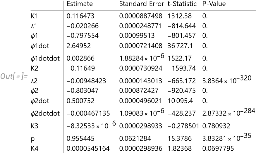
My previous answer dealt more with getting starting values. Once you have good starting values, then MultiNonlinearModelFit works fine. But I do need to give my standard caution: MultiNonlinearModelFit currently assumes a common error variance and that the residuals between the multiple models are all independent. That assumption is not always true.

nlmPitch = ResourceFunction["MultiNonlinearModelFit"][{Angle1, Angle2}, 
  {K1 E^(λ1 x) Cos[ϕ1 + ϕ1dot x + ϕ1dotdot*x^2/2] + 
     K2 E^(λ2 x) Cos[ϕ2 + ϕ2dot x + ϕ2dotdot*x^2/2] + K3 Cos[p x], 
   K1 E^(λ1 x) Sin[ϕ1 + ϕ1dot x + ϕ1dotdot*x^2/2] + 
     K2 E^(λ2 x) Sin[ϕ2 + ϕ2dot x + ϕ2dotdot*x^2/2] + K3 Sin[p x] + K4}, 
   {{K1, 0.1}, {λ1, -0.02}, {ϕ1, -0.8}, {ϕ1dot, 2.6}, {ϕ1dotdot, 0.003},
    {K2, -0.12}, {λ2, -0.001}, {ϕ2, -0.8}, {ϕ2dot, 0.5}, {ϕ2dotdot, -0.0005},
    {K3, -0.00003}, {p, 1.1}, {K4, 0.00006}}, x];
nlmPitch["ParameterTable"]

ParameterTable

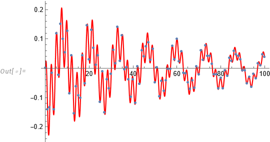
Show[Plot[nlmPitch[1, x], {x, 0, 100}, PlotStyle -> Red], ListPlot[Angle1]]

Angle1 and fit

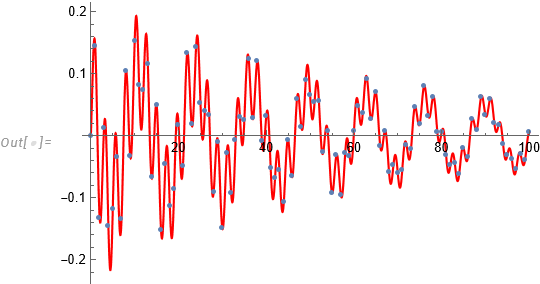
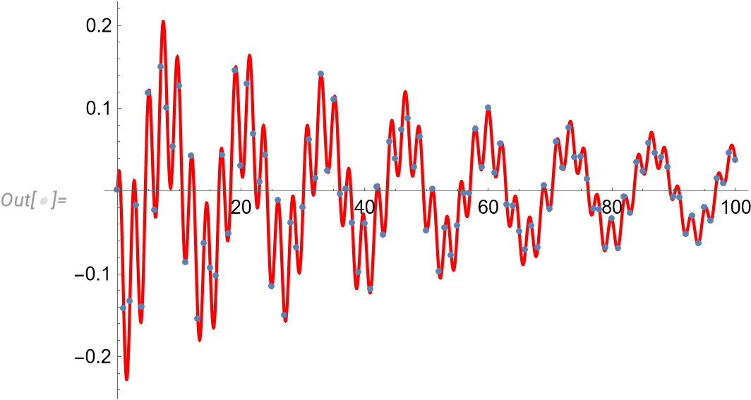
Show[Plot[nlmPitch[2, x], {x, 0, 100}, PlotStyle -> Red], ListPlot[Angle2]]

Angle2 and fit

$\endgroup$
2
  • $\begingroup$ Thank you for this answer @JimB. ϕ1dot and ϕ2dot are supposed to capture a slow oscillation (precession) and fast oscillation (nutation) respectively. Could you briefly explain how you chose the initial values in the answer above? In the new correlation matrix I see several less ones than before, however there are some left. Do you still think the ansatz suffer from too many parameters? This post gained significantly more attention that I first anticipated, so I'm still digesting the load of good answers and comments i received. $\endgroup$
    – MOOSE
    Commented Jul 27, 2022 at 6:31
  • $\begingroup$ Not knowing the physics, I just tried separating the starting values of $\phi$dot1 and $phi$dot2 by a bit and hoped for the best. The only "1's" left are on the diagonal which just means the parameter estimators are perfectly correlated with themselves. $\endgroup$
    – JimB
    Commented Jul 27, 2022 at 20:55
5
$\begingroup$

This is an extended comment (as it requires some graphs).

  1. Plot your data.
  2. Good starting values are your best friends (as mentioned by others).
  3. Each dataset of yours is capable of estimating all of the parameters for its associated model so after getting good starting values, fit each model separately. Then go to MultiNonlinearModelFit.
  4. Consider starting out with simpler models and then building in more complexity.

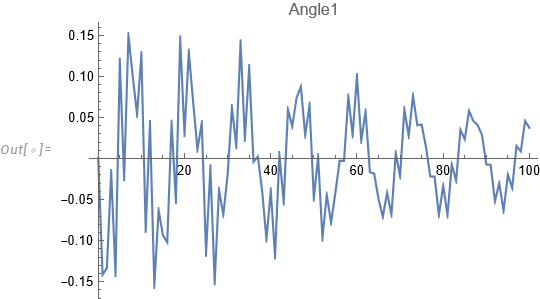
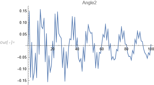
A plot of the data with the data points connected shows the following:

ListPlot[Angle1, Joined -> True, PlotLabel -> "Angle1"]

Plot of Angle1 dataset

ListPlot[Angle2, Joined -> True, PlotLabel -> "Angle2"]

Plot of Angle2 data

I'll just concentrate on the Angle1 data.

The model for Angle1 is

model1 = K1 E^(λ1 x) Cos[ϕ1 + ϕ1dot x + ϕ1dotdot*x^2/2] +
  K2 E^(λ2 x) Cos[ϕ2 + ϕ2dot x + ϕ2dotdot*x^2/2] + K3 Cos[p x]

We see that there are 8 peaks across the 100 units so a reasonable starting value for both ϕ1dot and ϕ2dot is around 0.5:

Solve[f 100 == 8 2 \[Pi], f] // N
(* {{f -> 0.502655}} *)

The heights of the peaks start at around 0.15 and drop to around 0.07. That suggests a starting value for both λ1 and λ1 of around -0.008:

Solve[Exp[λ1*100] == 0.07/0.15, λ1, Reals] // Quiet
(* {{λ1 -> -0.0076214}} *)

The heights of the peaks start at around 0.15 so that would be a reasonable starting value for K1, K2, and K3. For the remaining parameters, I'd give zero as the starting value. (Others might see things in the data which would work better than 0.)

Putting this altogether:

model1 = K1 E^(λ1 x) Cos[ϕ1 + ϕ1dot x + ϕ1dotdot*x^2/2] +
  K2 E^(λ2 x) Cos[ϕ2 + ϕ2dot x + ϕ2dotdot*x^2/2] + K3 Cos[p x]
nlm1 = NonlinearModelFit[Angle1, model1, {{K1, 0.15}, {λ1, -0.008}, {ϕ1, 0}, 
  {ϕ1dot, 0.5}, {ϕ1dotdot, 0}, {K2, 0.15}, {λ2, -0.008}, {ϕ2, 0}, {ϕ2dot, 0.5}, 
  {ϕ2dotdot, 0}, {K3, 0.15}, {p, 0}}, x, MaxIterations -> 5000];
Show[ListPlot[Angle1, Joined -> True], 
 Plot[nlm1[x], {x, 0, 100}, PlotStyle -> Red]]

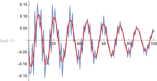
Data and fit for Angle1 data

Looks like a reasonable fit but your troubles aren't over. A look at the parameter correlation matrix results in several correlations among the parameters being 1 and a few more very close to -1. This means that while your model makes reasonable predictions, it is way over-parameterized. You need either a simpler model or more data that can estimate the parameters without the perfect correlation.

NumberForm[nlm1["CorrelationMatrix"] // MatrixForm, 3]

Parameter correlation matix

If all you need is a prediction, then maybe everything is OK. But if you need to interpret individual coefficients, then you're in trouble. Might fitting the two models simultaneously fix the perfect correlation issue? It's possible but I doubt it. Good luck!

Update:

@user293787 pointed out that giving the same starting values for ϕ1dot and ϕ2dot might cause NonlinearModelFit to end up with the wrong estimates which could explain the high correlations among the parameter estimators. That turns out to be the case. Here's an updated fit. I simply separated the two starting values, chose 1 for the starting value of p, and found that MaxIterations -> 5000 could be removed:

model1 = K1 E^(λ1 x) Cos[ϕ1 + ϕ1dot x + ϕ1dotdot*x^2/2] +
  K2 E^(λ2 x) Cos[ϕ2 + ϕ2dot x + ϕ2dotdot*x^2/2] + K3 Cos[p x]
nlm1 = NonlinearModelFit[Angle1, model1, {{K1, 0.15}, {λ1, -0.008}, {ϕ1, 
    0}, 
  {ϕ1dot, 0.8}, {ϕ1dotdot, 0}, {K2, 0.15}, {λ2, -0.008}, {ϕ2, 0}, 
  {ϕ2dot, 0.3}, {ϕ2dotdot, 0}, {K3, 0.15}, {p, 1}}, x]
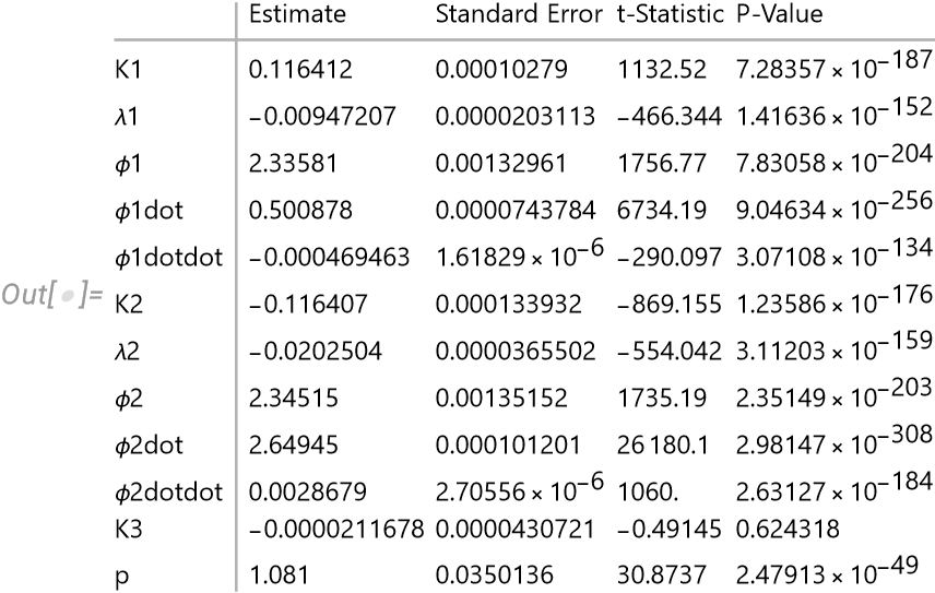
nlm1["ParameterTable"]

Parameter table for model1

It appears that the K3 Cos[p x] can be dropped (by looking at the difference in the AICc values.

Show[Plot[nlm1[x], {x, 0, 100}, PlotStyle -> Red], ListPlot[Angle1]]

Angle1 data and new fit

$\endgroup$
2
  • 1
    $\begingroup$ You used equal starting values for ϕ1dot and ϕ2dot. Presumably ϕ2dot is supposed to capture the residual higher frequency "zig zag" structure in the data that I think one can sort of see in your last plot. That might resolve some of the correlation problem that you point out. $\endgroup$
    – user293787
    Commented Jul 25, 2022 at 16:50
  • $\begingroup$ @user293787 Good point! And that does wonders for the fit. I'll update my answer. $\endgroup$
    – JimB
    Commented Jul 25, 2022 at 17:17
2
$\begingroup$

Not an answer, but an observation to think further.

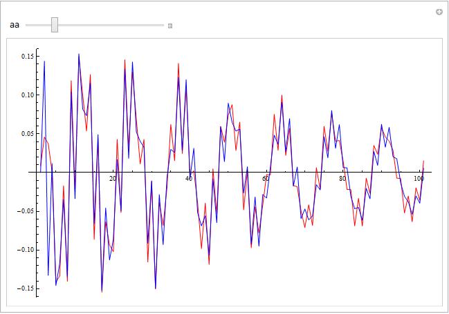
Seems Angle1 shifted 3 m to right is Angle2 plus litte noise !?

Manipulate[
 ListLinePlot[{RotateLeft[Last[Transpose[Angle1]], aa], 
   Last[Transpose[Angle2]]}, PlotStyle -> {Red, Blue}, 
  ImageSize -> 600], {{aa, -3}, -5, 5, 1}]

enter image description here

Manipulate[
 ListLinePlot[{RotateLeft[Last[Transpose[Angle1]], aa] - 
    Last[Transpose[Angle2]]}, PlotStyle -> {Red, Blue}, 
  ImageSize -> 500, GridLines -> Automatic, 
  PlotRange -> {-.3, .3}], {{aa, -3}, -10, 10, 1}]

Observe further interesting behaviour for aa =-5 or aa = 4. Leave it to you to interpret.

$\endgroup$
4
  • $\begingroup$ +1 Good observation. Correlation[Transpose[{Angle1[[4 ;; 100, 2]], Angle2[[1 ;; 97, 2]]}]] = -0.974159. While the parameter estimates might not change much if this more complicated error structure is considered, it does leave the standard errors as being likely too small. $\endgroup$
    – JimB
    Commented Jul 25, 2022 at 19:22
  • $\begingroup$ One more comment on this: if Angles2 is fit with model1, then all estimated coefficients are nearly identical except for one phase parameter. $\endgroup$
    – JimB
    Commented Jul 25, 2022 at 21:02
  • $\begingroup$ To me it makes physical sense than angle1 and angle2 should be similar due to that it is supposed to describe an epicyclic (maybe tricyclic) motion. That is the motion is supposed to look like a gyroscopic motion with both precession and nutation. If there were more datapoints in between the 1 meter spacing we would be able to see this more continously through ListPlot[Transpose@{Pitch1m[[1 ;; n, 2]], Yaw1m[[1 ;; n, 2]]}] $\endgroup$
    – MOOSE
    Commented Jul 26, 2022 at 7:33
  • $\begingroup$ Dear MOOSE , it would be essential to know, how exact your data are, means what are the measurement errors? Further, are there systematic measurement errors, which could explain the behaviour at aa=5 or 4? Is this noise in my picture above, or, if not, the soffisticated answer of @JimB shows the right way. $\endgroup$
    – Akku14
    Commented Jul 27, 2022 at 3:24
1
$\begingroup$

Just a side comment around the starting values. For these type of multi-function fits, I usually define my chi-squared merit function and minimise it using NMinimize.

For this case the function looks like this:

chiSquare = 
  Total[(Table[(K1 E^(\[Lambda]1 x) Cos[\[Phi]1 + \[Phi]1dot x + \
\[Phi]1dotdot*x^2/2] + 
         K2 E^(\[Lambda]2 x) Cos[\[Phi]2 + \[Phi]2dot x + \
\[Phi]2dotdot*x^2/2] + K3 Cos[p x]), {x, Angle1[[All, 1]]}] - 
      Angle1[[All, 2]])^2] + 
   Total[(Table[(K1 E^(\[Lambda]1 x) Sin[\[Phi]1 + \[Phi]1dot x + \
\[Phi]1dotdot*x^2/2] + 
         K2 E^(\[Lambda]2 x) Sin[\[Phi]2 + \[Phi]2dot x + \
\[Phi]2dotdot*x^2/2] + K3 Sin[p x] + K4), {x, Angle2[[All, 1]]}] - 
      Angle2[[All, 2]])^2];

and the for minimisation process I use RandomSearch:

nmin = NMinimize[
  chiSquare, {K1, \[Lambda]1, \[Phi]1, \[Phi]1dot, \[Phi]1dotdot, 
   K2, \[Lambda]2, \[Phi]2, \[Phi]2dot, \[Phi]2dotdot, K3, p, 
   K4},Method -> {"RandomSearch", "SearchPoints" -> 50}]

yielding:

{0.00001689, {K1 -> -0.116492, [Lambda]1 -> -0.00948456, [Phi]1 ->
-0.803049, [Phi]1dot -> 0.500752, [Phi]1dotdot -> -0.000467153, K2 -> 0.116472, [Lambda]2 -> -0.0202657, [Phi]2 -> -0.797566,
[Phi]2dot -> 2.64952, [Phi]2dotdot -> 0.002866, K3 -> 0.0000286455, p -> -0.438194, K4 -> 0.0000544006}}

which you can check, by plotting the results, that it is a pretty good fit having an even better value of chi-square than that of the "MultiNonlinearModelFit" (which is 0.0000169157 if you check the ANOVAtable values, nlmPitch["ANOVATable"]. The difference of course is very small, 0.15%). The good thing of NMinimize function is that it has a plethora of solvers with many parameters that you can tune in order to locate the global minimum.

$\endgroup$
6
  • 1
    $\begingroup$ I agree that using NMinimize seems to be more numerically stable than not using it (which can be used in NonlinearModelFit by including Method->"NMinimize"). But where are the measures of precision for the individual parameters? $\endgroup$
    – JimB
    Commented Jul 27, 2022 at 20:48
  • $\begingroup$ This is only for the initial values. However, if you want to derive the various quantities (i.e. precision, parameter errors etc.) the super-correct way is to formulate the DeltaChiSquared values and start minimising it for various Deltas. Have a look here foo.be/docs-free/Numerical_Recipe_In_C/c15-6.pdf page 693. In this way you can inherently take into account non-gaussianity, data dependencies etc. yielding asymmetric errors as expected. This will is more robust than the standard method (i.e. the diagonal elements of the error matrix) provided by default by Mathematica and others $\endgroup$
    – demm
    Commented Jul 27, 2022 at 21:28
  • 1
    $\begingroup$ My concern/stereotype about producing just estimates is that many folks in physics and engineering produce estimates but don't always seem concerned about producing associated estimates of precision. And that book you mention explains why I see the prevalence of using "chisquared" statistics procedures as that book was written two physicists and not statisticians. I don't know why you say that minimizing a chisquared statistic makes things more robust. (Don't get me wrong: that book is an excellent reference.) $\endgroup$
    – JimB
    Commented Jul 27, 2022 at 21:42
  • $\begingroup$ I fully agree! I personally prefer maximum likelihood and Bayesian optimization taking into consideration (if possible the true underlying distribution). However, most of the ready-made fitting recipes (in Mathematica, Matlab, Python R etc.) are based on chi-square, including NonlinearModelFit and MultiNonlinearModelFit that are referenced in this question. Thus, if we decide to take the chi-square road then the DeltaChi square approach is more robust and in the case of gaussianity and independence it naturally converges to the diagonal of the error matrix (for the chi-square estimator!). $\endgroup$
    – demm
    Commented Jul 27, 2022 at 22:07
  • 1
    $\begingroup$ If only more direct Bayesian procedures were added to Mathematica! One can dream. $\endgroup$
    – JimB
    Commented Jul 27, 2022 at 23:30

Your Answer

By clicking “Post Your Answer”, you agree to our terms of service and acknowledge you have read our privacy policy.

Not the answer you're looking for? Browse other questions tagged or ask your own question.